CAR CRASH HOTSPOTS ANALYSIS IN WELLINGTON CITY

I. INTRODUCTION

1. Background

Road traffic accidents constitute a significant contributor to premature mortality, ranking tenth worldwide in incidence and ninth in Disability Adjusted Life Years (DALYs), whereas in high – income nations, they are the third leading cause of death (WHO,2000). Nonetheless, road traffic accident rates, whether assessed by population or distance traveled, are consistently declining in developed nations due to enhanced safety in roads and vehicles. In New Zealand, road traffic accidents continue to be a major concern despite progress in road safety measures. In 2022, 375 road deaths were recorded, marking a slight increase from previous years (ITF, 2023). Since road safety is a top priority, government’s Road to Zero strategy aiming for 40% reduction in deaths and serious injuries by 2030 (ITF, 2023).

2. Research Questions

Wellington is the mountainous terrain with serpentine roads and recurrent extreme weather conditions which usually include strong winds and heavy rainfall, this presents the distinct driving problems. According to (Wang et al., 2021), the presence road surface condition, road pavement condition were significant factors affecting the severity of vehicle. Moreover, as Wellington is the capital of New Zealand, this has high levels of both commuter traffic and tourism which might have a significant impact on road accidents especially during the peak hours which contribute to traffic congestion and accidents.

This report focusses on analyze the car crash at Wellington city, with mainly focus to answer two critical questions:

1. Where are the spatial hotspots of road traffic accidents in Wellington?
2. What are the key factors influencing the severity of road traffic accidents in Wellington?

In order to answer these two questions, this analysis uses data from the Crash Analysis System (CAS) which record all traffic crashes reported by the New Zealand police.

II. DATA AND METHODS

1. Data Overview

1.1 Crash Analysis System (CAS)

Crash severity is the most severely injured casualty occurring as a result of crash (Austroads, 2003). According to CAS data, the severity of a crash had been divided into 4 different types (table 1).

As serious car crashes and fatal often involves significant injuries or fatalities that usually result in severe consequences such as hospitalization and loss of life, we chosen to group serious crash and fatal crash into group. On the other hand, both non – injury crash and minor crash often share common characteristics such as lack of injuries and minimal need for medical attention, in order to make our analysis easy to interpret, this analysis only consider 2 types of crash: serious (include fatal) crash, non - injury crash.

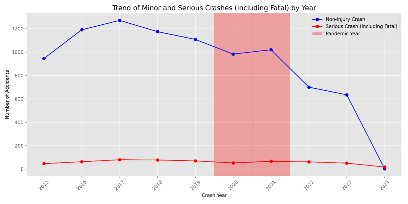
To make sure our research represents the latest period, we first considered relying exclusively on the last three years of our dataset of accidents. By looking at the yearly number of crashes, we decided that data was too sparse to do any meaningful model development since the number went down to only 1,338 cases of Non - Injury Crashes and 131 cases of Serious Crashes (include fatal). In light of this constraint, we extended the timeframe to the past decade (2015–2024), yielding a more substantial dataset (non - injury crashes: 9,031; serious crashes: 589), while still including the most current years. This decision guarantees sufficient data for the effective processing of the model. The figure below shown the Non – injury and Serious/Fatal crash at a chosen period (2015 – 2024).

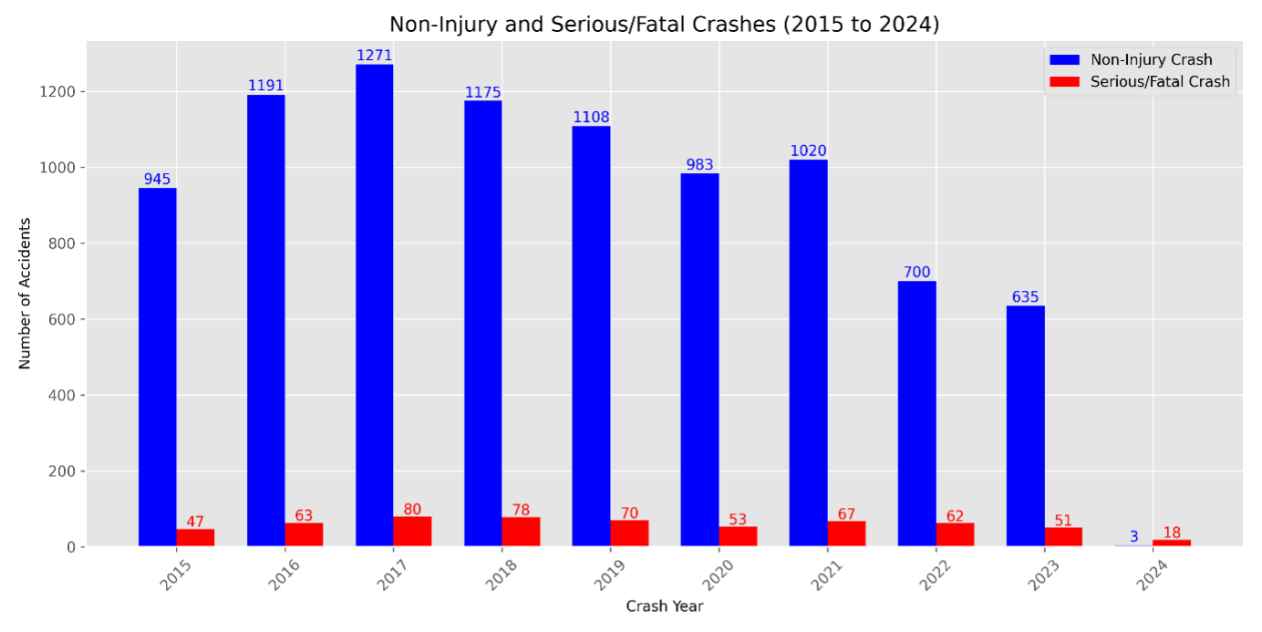
According to figure 01, although the COVID-19 pandemic influenced road traffic because of lockdowns, car crashes still happened during this period. Based on the trend from figure 02, non - injury crashes and serious crashes (including fatal), occurred at different levels during the pandemic years, 2020–2021. Continuity of crashes during the pandemic, therefore, only reinforces this period for incorporation into our analysis of car crashes. In other words, including the period of the pandemic into our analysis ensures that our study captures every form of behavior associated with crashes, including shifts resulting from outside events like COVID-19.

1.2 Wellington SA2 Dataset

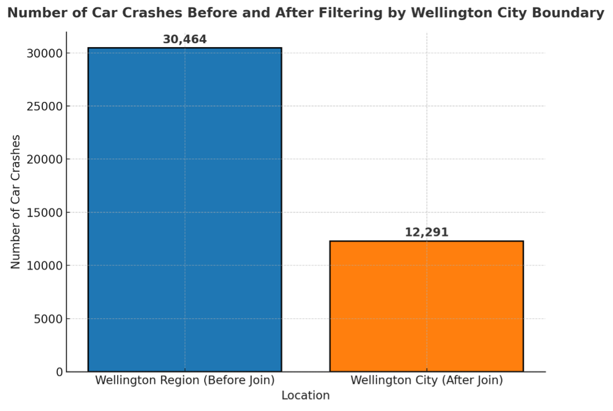
Our focus is car crashes within Wellington City; however, the raw dataset encompasses the entire Wellington region. So, we filtered out the points that were outside of Wellington City to make sure that we are analyzing only crashes within the city boundaries. For this purpose, we used the New Zealand territorial authority boundaries provided by StatsNZ, this dataset is the authoritative source for annually updated territorial boundaries. We filtered this crash data to include only those crashes that had a TA code for Wellington City. We performed another spatial join in order to clean this data set further and retain only car crashes that fell inside the Wellington City boundary. The plot below outlines how many car crashes existed before and after the spatial join was used. Originally there were 30,464 crashes in the Wellington region. After filtering, 12,291 crashes remained within Wellington City indicate that half of them was outside the city boundary.

1.3 Wellington Liquid Store Location

The use of alcohol alters driving performance even at low dosage levels (e.g. at blood alcohol levels, [BALs] as low as .02% [Moskowitz, Bums, and Williams 1985]). It has been indicted as affecting response times to dangerous road situations (West et al. 1993). According to (Heeren, et al. 1985 and Ostrom and Eriksson 1993), the majority of single-vehicle nighttime fatal crashes are alcohol involved. Based on previous research, the impact of alcohol retail seems to have a significant impact on the car crash, hence, we used the alcohol store location in Wellington city provided by OpenStreetMap to include in our analysis. This was performed by calculate the distance between the car crash and the alcohol store (using spatial nearest join) to identify the influence of liquor store on the crash.

2. METHODOLOGY

2.1 Spatial Hotspot Analysis

In this analysis, both Global and Local Moran's I will be implemented. Global Moran's I will determine the overall spatial autocorrelation to display whether accidents are dispersed, random, or clustered within the region. Local Moran's I on the other hand provide detailed information by highlight the distinct regions as clusters of high or low crash rates. Other papers looking at the spatial autocorrelation of crash frequencies also have used Moran’s I to investigate crash data at similar levels of spatial aggregation (Matkan et al., 2013). This article also used both Global and Local Moran’s I analysis to conclude the frequency and location of traffic incidents, global Moran’s I was used to highlight where clusters exist while Local Moran’s I was used to indicate the place and type of spatial autocorrelation. Finding regions with high or low rates of accidents and determining the extent of spatial autocorrelation in the data will be able to evaluate the specific regions which have a disproportionate number of crashes, this may warrant targeted road safety improvements. Figure 5 shows the hotspot analysis method that would be used in this analysis.

The data aggregation method will convert crash locations into spatially significant units by combining them into predefined polygons such as statistical regions or mesh blocks. This phase ensures the appropriate spatial units for conducting Moran's I analysis. This aggregation is essential for guaranteeing that the hotspot analysis results are statistically sound and spatially interpretable. Prior research has employed the Traffic Analysis Zone (TAZ) as the analytical spatial unit (Soltani & Askari, 2017). We have chosen to utilize the SA2 unit level for analysis in our study, as it is comparable in size to the TAZ used in prior research. We have opted to utilize the SA2 level for data aggregation, since it will render hotspots discernible and interpretable, given that SA2 zones are delineated by roads and are sufficiently large to be represented on a map of Wellington.

Kernel Density Estimation

Kernel Density Estimation (KDE) is a widely utilized technique for analyzing the first-order characteristics of a point event distribution (Bailey & Gatrell, 1995; Silverman, 1986), mostly due to its simplicity and ease of implementation. The purpose of KDE is to produce a smooth density surface of point events over space by computing event intensity as density estimation. Hence, in our study, before data is aggregated to the SA2 polygons for analysis, the points can be turned into a KDE surface to understand basic patterns and areas with high accident rates. This has previously been used as a tool for finding hotspots in other crash research and in some cases has outperformed other spatial models (Hashimoto, et al. 2016). These KDE maps can be used to get an initial idea of where hot or cold spots may occur within Wellington before deeper statistical analysis.

3. Model

In the following analysis, we want to find which of the variables have significant effects on the magnitude of automotive crashes. We will take the target variable as a binary class: 0-Non-Injury Crashes, 1-Serious/Fatal Crashes. We merged Serious and Fatal Crashes into one category (as mentioned below). Excluding Minor Crashes would provide a sharper contrast between the classes since minor crashes are in a gray area that may obscure an analysis. The major model building process is shown in Figure 5 below.

3.1 Feature Selection

The independent variables selected for this model include flatHill (Whether the road is flat or sloped), light (lighting conditions), roadSurface (surface condition sealed or not), speed limit, intersection and two weather-related variables, weatherA(rain, snow, mist), weatherB(frost, wind) and distance to alcohol store. These variables are informed by prior research, ensuring relevance to crash severity. For instance, Edwards (1998) compared accident severity across adverse weather conditions such as rain, fog, and wind against fine weather. Similarly, Bazzanaa et al. (2019) explored how speed enforcement systems influence accidents on highways. Lighting conditions are also significant; Jackett and Frith (2013) highlighted a 35% reduction in crashes when lighting was improved, according to the NZTA Economic Evaluation Manual. Further, Lee et al. (2015) and Hosseinpour et al. (2014) found that factors such as road surface conditions and horizontal curvature are linked to more severe crashes. The study from (GRUENEWALD & PONICKI, 1995) strongly support greater overall use of alcohol is related to greater likelihoods of death in alcohol-involved crashes.

3.2 Data Cleaning

Addressing missing data is another crucial step. During the exploratory phase, we found that the intersection data had a 100% missing rate. To resolve this, we sourced intersection data from Wellington’s records, which allows us to impute the missing values and maintain data integrity for our model.

3.3 Handling Class Imbalance

A problem associated with our dataset of car crashes in Wellington over the last 10 years is the huge class imbalance. The ratio of Non-Injury to Serious/Fatal crashes is about 15:1; less than 1% of the data is of the positive class. Such a skewed class balance can bias the model toward negativity and hence neglect the patterns that correspond to more serious crashes. In balancing this, we apply down-sampling to the negative class to get a 4:1 ratio. The selection is informed by research of (Mehdi 2013), who used similar ratios for crash severity analysis, and (Tom Williams, 2018), who applied this in modelling bicycle-motor vehicle crashes in Christchurch.

3.4 Logistic Regression Model

First, we apply a Standard Logistic Regression model to predict crash severity. However, the inherent spatial nature in car crashes requires us to check whether a spatial pattern in the residuals is driving the model. If Moran's I detect some spatial autocorrelation, then this may mean that the location itself plays a role in the crash severity not captured by the variables themselves. Then we might need Geographical Weight Logistic Regression (GWLR) model to see if this better fit by comparing the AUROC and Pseudo R – squared.

III. RESULTS & DISCUSSION

1. Result

1.1 Kernel Density Estimation (KDE)

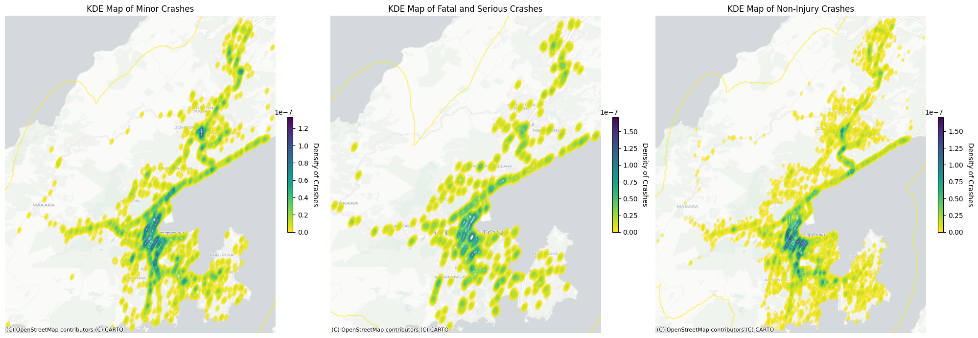
The KDE maps above show the density distribution of crashes across wellington city for each of the 3 different crash types. For All three crash types we see the highest density of crashes is occurring in the city centre.

1.2 Spatial Autocorrelation

1.2.1 Global Moran's I

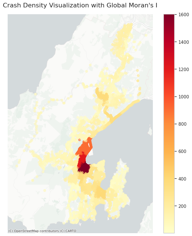
The Global Moran’s I test determines if there is spatial autocorrelation present in the crash data across wellington city. The map show here highlights the density of crashes seen across Wellington city for the entire data sets and what areas might see more clustering.

1.2.2 Local Moran's I

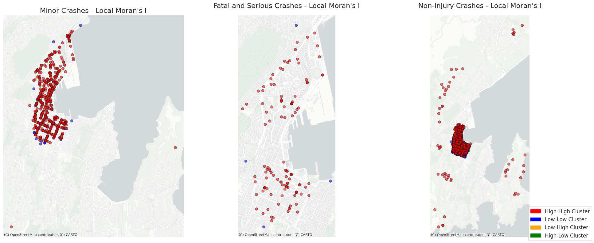
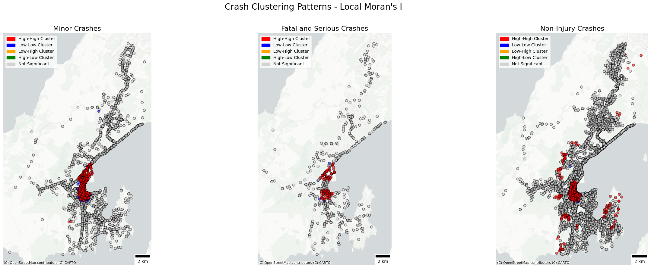
Local Moran’s I was used to identify the specific locations of hot and cold spots of crashes for minor, fatal and serious, as well as non-injury crashes. Within a dataset, local Moran's I aid in locating hotspots and cold spots or clusters of high and low values. We did this process after assessing the global metrics of the entire crash dataset with Global Moran's I. The Maps above highlight the hot and cold spots and specific local clusters for each crash type. Below, we removed non-significant crash points to better see the high and low clusters. The weighting method used above was K Nearest Neighbor with the K value or number of neighbors set to 5. The K values choice of 5 was utilized in this weighting method to focus on Local hotspots of crashes without hotspots becoming to generalized or determined by small scale changes in crash density. Studies have highlighted the importance of this variable selection as the findings are strongly impacted by the choice of KNN that differs by several units (Kubara & Kopczewska, 2024). For the context of our study using a smaller number is preferable as we want to focus on smaller hotspot areas of crashes within Wellington. The KNN method has been used in other studies and was determined as a viable weighting method especially for road crash incident analysis (Sahu et al., 2023).

1.3 Classification Model

In the exploratory data analysis, we found that the intersection variable contained all missing values. So it’s removed in the model stage. Furthermore, since six out of the seven variables are categorical, we examined the distribution of these variables and their relationships with the dependent variable, as shown in Table 1 below:

The results of the logistic regression model are shown in Table 2 below. We transformed the categorical features into one-hot encoded variables by using dummy variables. The Pseudo R² is 0.1148, and the AUROC is 0.64. We report Nagelkerke R² because it is commonly used in logistic regression outputs and is conceptually similar to the R² in linear regression while it’s generally lower than R² in linear regression. Among the categorical variables, "light," "speed limit," "weather A," and "weather B" have significant coefficients compared to their default value. Additionally, the only continuous variable "distance to store (km)" also has a significant coefficient.

2. DISCUSSION

2.1 Kernel Density Estimation (KDE)

When looking at the KDE maps in Figure 6 all three crash types saw the highest density of crashes in the center city. This is especially true for minor and non-injury crashes. Fatal crashes have a notably lower density in the city center when compared to the other minor and non-injury crashes. We also see a main road and highway segments have smaller hotspots of crashes along them for all three crash types. The KDE maps above give us an overall view of the distribution of crashes for each type before we do further statistical analysis.

2.2 Global Moran's I

When looking at the amp above in Figure 7 the test produces a Global Moran’s I result of 0.9784 (4DP) which means that the data indicates strong positive spatial autocorrelation. In terms of our data and investigation this means that we should see areas of high crash counts should be located next to other areas of high crash counts. The test also obtained a Z score of 185.73 which is very high. This indicates that level of clustering seen is very significant and is much higher than we would expect to see under random conditions. The Z score is large enough to say that there is very strong evidence of clustering within the data.

2.3 Local Moran's I

When looking at the clustering results from LISA maps above in Figure 8 we can see a few key differences in the clustering for each crash type. Non-injury crashes had the widest dispersion of high-high clusters. Minor crashes had significant high-high clusters almost exclusively within the center city. Fatal and serious crashes had high-high and a handful of low-low clusters outside of the main CBD area. It is important to note that we do not see outlier clusters (Low-High and High-Low) for several reasons. Firstly, we saw a very strong P value during the Global Moran’s I am meaning that the data has very strong spatial autocorrelation of the crash points. These HL and LH cluster may not exist at the specified threshold set for the LISA clusters. Additionally, because the crash data points were abundant in terms of sample size we may see a large amount of spatial heterogeneity in the data. These spatial cluster we see do align with the density cluster fund in KDE earlier in the spatial analysis process.

2.4 Logistic Regression Model

The Pseudo R² value of 0.1148 shows approximately 11.5% of the variation in dependent variable (crash severity) is explained by the model. In logistic regression, a Pseudo R² below 0.2 is usually considered a weak explanation of dependent variable. Therefore, our model shows limited explanatory power. Compared to a similar study on bike crash severity in Christchurch, which has Pseudo R² values ranging from 0.3 to 0.6, our model's performance is relatively poor. This suggests that the variables included in our model may not be the primary factors influencing crash severity. Additionally, the AUROC for the test data is 0.64 which means the model has limited ability to distinguish between classes. Normally, closer to 0.5 is regarded as the same as random classification, while above 0.7 is usually considered as acceptable model performance.

Even though the model doesn’t have a good performance in prediction level, our primary focus is on understanding the significance and direction of the influence of selected variables on crash severity. Based on the model summary, we could say that compared to bright sunlight, overcast conditions would decrease the likelihood of a serious crash. Compared to 30 km/h or below, mid or high-speed limits would increase the likelihood of serious crashes. As for weather conditions, rainy, misty, or foggy weather does not significantly increase the likelihood of serious crashes compared to the clear weather. On the other hand, strong winds weather compared to unknown wind or frost weather would increase likelihood of serious crashes which might worth noticing since the Wellington city is quite windy. Additionally, when car crash location’s distance from a liquor store increases, the likelihood of a serious crash also increases.

2.5 Unsual Correlation

There are a few unusual correlations between serious crashes and spatial factors in our model. One unexpected result is the significant negative relationship between mid and high-speed limits and serious crashes. This suggests that roads with higher speed limits are associated with fewer serious crashes. This means that the low-speed limit (30 km/h or below) is usually found in specific scenario like roadwork zones. A possible explanation could be that there aren’t enough clear signs for drivers to slow down or drivers are careless with the sign and fail to slow down accordingly in these areas.

Another surprising finding is that the distance to liquor stores has a positive significant relationship with serious crashes, meaning that crashes are more likely to be serious when they occur farther from a liquor store. This may be due to a limitation in our data source since we only collected data from 14 liquor stores in Wellington, most of which are in the central business district (CBD). If crashes are more likely to be more serious in the highway which are more likely to be away from CBD, this could explain the positive relationship between distance to liquor stores and crash severity.

2.6 Spatial Autocorrelation Detection

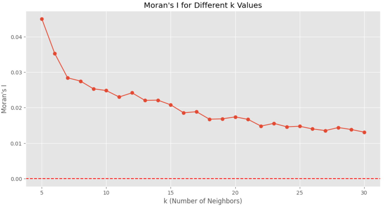
Since in the hotspot analysis showed significant spatial autocorrelation, it's important to check whether this violates the assumption of no spatial autocorrelation in our logistic regression model. Some variables might not be significant at the global level, but it might not be the same in local level. So we need to assess whether the residuals are spatially autocorrelated. This would help us decide whether we should use a geographically weighted logistic regression (GWLR) for local-level analysis. Since we are working with logistic regression instead of linear regression, we used deviance residuals which measure the difference between the predicted probabilities and the actual outcomes with penalty in difference. To avoid bias from the random splitting of data, we re-ran the model on the entire dataset to ensure the spatial location of observations is fully considered. To check for spatial autocorrelation, we used the k-nearest neighbors (KNN) method to calculate Moran’s I for the deviance residuals. Because the choice of k can influence the results of Moran I, we tested a range of k-values from 5 to 30. The Moran’s I values are shown in the figure below. Although all Moran’s I values are statistically significant at the 0.05 level, the strength of autocorrelation is very weak across all k-values. Since the spatial autocorrelation is weak, we can conclude that the significance of the model's coefficients is not due to spatial autocorrelation. As a result, it suggests that a geographically weighted model is not necessary here.

IV. LIMITATIONS AND FUTURE WORK

1. Limitations

A main limitation is that some key variables that are likely to be important in predicting the severity of crashes were not included. For instance, intersections are a very critical factor concerning severe crashes. However, the intersections column in the car crash dataset is missing. We looked for alternative data about intersections, but none was available, and due to the limit of time we couldn’t create accurate version by ourselves. Similarly, we had don’t have the type of road data which is important road features in car crash. Even though some information was found from NZTA showing the hierarchy of the roads, there aren’t geometry data available. Spatial variables distance to liquor store for our model may not be accurate defined since most of the liquor stores are in the CBD and this could have a biased outcome because it might not be representative of the rural area. The downsampling method could also introduce bias since downsampling doesn't consider the spatial distribution of the crashes, it may distort the location distribution. Besides, it should have been comparison between sampled and whole dataset to see if such an effect exists.

2. Future Work

Even though our analysis target is to understand if the selected feature is significant in influencing the severity of car crash, further work could still focus on finding key factors that explain more of the variant of serious crashes for policy advice and improve the model performance like Pseudo R². For example, including key factors like intersection and road type data might help explain the variation in crash severity as they are significant factors in another research. Furthermore, we could explore and include more variables like “distance to liquor store” that might help better capture the relationship between drunk driving and crash severity.

V. CONCLUSION

In conclusion, the analysis revealed significant spatial autocorrelation in road traffic accidents within Wellington which highlighting hotspot areas in the city center. Several factors such as weather conditions, speed limits, and distance to liquor stores were found to influence crash severity though the logistic regression model While the model provided insights into key factors affecting crash severity, further development might need to improve model accuracy such as including additional variables like intersections and road types.

THANK YOU FOR READING!

REFERENCES

1. WHO, 2000. World Health Organisation Report 1999. World Health Organisation, Geneva.
2. International Transport Forum (ITF). (2023). Road Safety Country Profiles New Zealand 2023.
3. Austroads. (2003). Austroads Guide to Traffic Engineering Practice. Part 4. Treatment of Crash Locations. https://www.nzta.govt.nz/assets/resources/guide-to-treatment-of-crash-location/docs/definitions.pdf
4. Wang, K., Zhang, W., Jin, L., Feng, Z., Zhu, D., Cong, H., & Yu, H. (2021). Diagnostic analysis of environmental factors affecting the severity of traffic crashes: From the perspective of pedestrian–vehicle and vehicle–vehicle collisions. Traffic Injury Prevention, 23(1), 17–22. https://doi.org/10.1080/15389588.2021.1995602
5. Moskowitz, H., Burns, M. and Williams, A. F. Skills performance at low blood alcohol levels. Journal of Studies on Alcohol, 46, 482-485, 1985.
6. West, R.; Wilding, J.; French, D.; Kemp, R.; Irving, A. Effect of low and moderate doses of alcohol on driving hazard perception latency and driving speed. Addiction, 88, 527-532, 1993.
7. Heeren, T.; Smith, R. A.; Moorlock, S.; Hingson, R. W. Surrogate measures of alcohol involvement in fatal crashes: Are conventional indicators adequate? Journal of Safety Research, 16, 127-134; 1985.
8. Ostrom, M.; Eriksson, A. Single-vehicle crashes and alcohol: A retrospective study of passenger car fatalities in northern Sweden. Accident Analysis and Prevention, 25, 171-176; 1993.
9. Matkan, A. A., Mohaymany, A. S., Shahri, M., & Mirbagheri, B. (2013). Detecting the spatial-temporal autocorrelation among crash frequencies in urban areas. Canadian Journal of Civil Engineering, 40(3), 195-203.
10. Trevor C. Bailey and Anthony C. Gatrell. Essex, England: Longman Scientific & Technical, 1995. xiv, 413 pp. ISBN 0582-24493-5.
11. Silverman, B. W. (1986). Density estimation for statistics and data analysis. London: Chapman Hall.
12. Hashimoto, S., Yoshiki, S., Saeki, R., Mimura, Y., Ando, R., & Nanba, S. (2016). Development and application of traffic accident density estimation models using kernel density estimation. Journal of Traffic and Transportation Engineering (English edition), 3(3), 262-270.
13. Edwards, J. B. (1998). The relationship between road accident severity and recorded weather. Journal of Safety Research, 29(4), 249-262.
14. Bazzanaa, F., Borsatia, M., & Cascaranoa, M. The role of average speed enforcement systems in preventing highway accidents: evidence from Italy.
15. Jackett, M., & Frith, W. (2013). Quantifying the impact of road lighting on road safety—A New Zealand Study. IATSS Research, 36(2), 139-145.
16. Lee, J., Nam, B., & Abdel-Aty, M. (2015). Effects of pavement surface conditions on traffic crash severity. Journal of Transportation Engineering, 141(10), 04015020.
17. Hosseinpour, M., Yahaya, A. S., & Sadullah, A. F. (2014). Exploring the effects of roadway characteristics on the frequency and severity of head-on crashes: Case studies from Malaysian Federal Roads. Accident Analysis & Prevention, 62, 209-222.
18. GRUENEWALD, P. J., & PONICKI, W. R. (1995). THE RELATIONSHIP OF Accident Analysis and Prevention, 21(2), 249-259.
19. Williams, T., Doscher, C., & Page, S. (2018). Spatial characteristics of bicycle–motor vehicle crashes in Christchurch, New Zealand. Journal of Transport and Land Use, 11(1), 849-864.
20. Sahu, S., Maram, B., Gampala, V., & Daniya, T. (2023). Analysis of Road Accidents Prediction and Interpretation Using KNN Classification Model (Vol. 490). Springer Nature Singapore. https://doi.org/10.1007/978-981-19-4052-1_18
21. Kubara, M., & Kopczewska, K. (2024). Akaike information criterion in choosing the optimal k-nearest neighbours of the spatial weight matrix. Spatial Economic Analysis, 19(1), 73–91. https://doi.org/10.1080/17421772.2023.2176539