🎶 Million Songs Dataset Project with PySpark 🎼

Background

The Million Song Dataset (MSD) is a comprehensive collection of data designed to foster music information retrieval research. Created by The Echo Nest and LabROSA, the dataset provides metadata and detailed audio features for one million songs, including song ID, track ID, artist ID, and various audio properties. Additionally, the dataset integrates user-song play counts and genre annotations from several sources. In this assignment we will focuses on exploring audio features and collaborative filtering to build classification models and song recommendation systems.

PART I: PROCESSING

1. Structure of MSD dataset

The Million Song Dataset was stored in the Hadoop Distributed File System (HDFS). The datasets are organized into various directories such as “Audio”, “Genre”, “Main”, “Tasteprofile”. Each of the directories contains multiple files as detailed in the directory tree (Appendix A). The table below provide the information on the file sizes, format, data type and number of rows for each dataset.

The overall size of the MSD dataset is 12.9 GB, which accounts for the actual size of the data in the dataset, while 103.5 GB accounts for the replication across HDFS. To give a better overview over the differences of datasets, sizes were converted into consistent units and their percentages were calculated. According to the table above, "Audio" is the biggest share in the dataset, accounting for 94.65%, while the "Tasteprofile dataset" shares 3.8% of the total size. About "Audio" there are three subdirectories: "Attributes", "Features", and "Statistics”, the data stored in all the files from "Attributes" and "Statistics" consists of strings in CSV format, while "Features" contains both string and numeric data, compressed in CSV.gz format. Finally, the "Tasteprofile" directory is divided into "Mismatches," consisting of string data in two text files, and "Triplets.tsv," containing string and numeric data in TSV format with eight compressed files. Furthermore, the "Genre" directory has three TSVs of string type while the "Summary" subdirectory inside "Main" contains two CSV files compressed with both numeric and string data each.

2. Number of rows in each dataset

Before counting the rows for each file in the dataset, several compressed files had to be decompressed using the “gunzip” command in HDFS. Based on table 1, the “Tasteprofile” directory have the highest number of rows at 48,393,618 accounts for 73.97% of the total rows over MSD dataset. Following by the “Audio” directory which contain 13,924,662 accounts for 21.28%. Other directory has less than 10% of rows contribute to the overall. Since this is the million-song dataset, we expect there should be the million rows for each feature dataset, however, all of the feature dataset is slightly less than 1 million. Therefore, if we want to perform the join to get the genre label this will get smaller than million songs as the genre count larger than the song count in a particular feature dataset.

3. A brief summary of the information contained in audio attributes datasets

The audio attributes datasets contain metadata which describe the structure of the audio features, this has two columns, the first column represent the name of feature data and the second column corresponding their data types. For example, the attribute names “Area_Method_of_Moment_1” are paired with the real data which typically mapped to “DoubleType” in Spark. This metadata will be used for defining the schema to the audio feature data. On the other hand, the audio feature dataset contains the actual audio data with rows represent different audio samples and there corresponding “track_id” at the end of each row. The feature data needs a schema that will defines the structure for each column, which is where the information from the attribute dataset comes into play. Keeping these two datasets separate we can maintain a clear distinction between metadata and data which makes the loading and processing the audio features easier. Moreover, metadata can be reused by feature datasets that contain the same type of attributes.

4. Explanation of how to create the StructType automatically

In order to create an automatically StructType, first, we define a dictionary called dict_type with mapping attribute types such as real and string to their corresponding Spark SQL types which DoubleType and StringType. By reading a specific dataset such as “msd-jmir-area-of-moments-all-v1.0”, we define a “generate_schema” function to create a schema by iterating through a data frame of attribute names and types. For each attribute, the function will look up the type in the dict_type that create above then it creates a StructField. These fields are collected into a StructType which represent the schema of the feature dataset. The attributes data was then loaded from HDFS which convert to a data frame and pass into the “generate_schema” function, this will automatically map each attribute to its correct data type. By using this schema, the feature dataset is loaded subsequently, and all columns are properly typed based on the attribute descriptions.

5.Explanation of the convenient in audio features & attribute names to use as column names

5.1 The advantages and disadvantages of using these column names

Since the column from the area of moment dataset that we have loaded above have a very long column name (e.g. Area_Method_of_Moments_Overall_Standard_Deviation_1), it would be useful during the initial exploration of the dataset as it offers transparency and make it easy for us to understand what each feature represents without external documentation. However, we might find it difficult when using these columns names to next steps such as training the model as we have to explore correlation between these columns and doing some feature selection and visualization. Therefore, it would be easier to interpret and observe if we rename these columns shorter and more compact, useful to discuss them when it comes to explanation data analysis and training model.

5.2 Explanation of how to rename columns in the audio feature datasets

In order to make the column easy to interpret and visualize, we developed a systematic approach to rename the columns in the audio feature dataset by mapping each dataset to a specific prefix and applying a consistent naming convention. First, we defined a list of dataset names and mapped each one to a corresponding prefix. For each dataset, we dynamically read both attributes and features files in HDFS and pass them through the schema function (as discuss below). For the first 10 columns, we appended the prefix followed by “std” and a sequential number as it indicates the standard deviation. For the next 10 columns, we used the prefix followed by “avg” as it represents for the average. The columns start with "MSD_TRACKID” and “track_id” will be keep the same as it considers as they serve as key columns for potential joins.

PART II: AUDIO SIMILARITY

1. Summary of the specific audio features dataset you have chosen

The 'area of moments' dataset extracts statistical moments from audio signals, treating them as a 2- dimensional function, similar to how moments are used in image processing (Fujinaga, 1996). These moments capture essential characteristics of the audio, such as texture and distribution patterns. Hence, we chose this dataset because it provides a comprehensive summary of the signal's properties, which is particularly useful for tasks like audio classification (Ajoodha et al., 2015). The AOM dataset contain 994,623 rows and 21 columns. The first 20 columns are numeric and represent statistical summaries of the audio signal, with the first 10 columns capturing the standard deviation and the next 10 columns representing the average. The final column, "MSD_TRACKID” is a string type that uniquely identifies each track. Since this feature dataset have a long column name, in order to make it easy to interpret and visualize, we create a systematic way to rename columns as below:

2. Generate the descriptive statistics for each audio features

2.1 Descriptive statistics

Before performing the descriptive statistics, it is important to check for missing values as they can affect the accuracy of the results. By using the “isNull()” function, we found 19 missing values in columns “AMM_avg_3” to “AMM_avg20”. Since this is a small portion of the overall data, we drop these rows to ensure a cleaner analysis. Moreover, we also drop the "MSD_TRACKID” as it is the track id column which shown no meaning in the descriptive statistics. The “describe()” function is used to perform a descriptive statistics and the result had been converted to Pandas dataframe with transposed the feature into rows for easy observe as there are too many columns.

The descriptive statistics shown all features have the same number of counts, with the minimum value at “AMM_avg_5” and maximum value at “AMM_avg_8”. The mean and standard deviation show varying ranges across feature, with some low value to extremely high of variability. This mean that some features show a wider range of value which is easy to capture the different between songs in different genres. On the other hand, several features with low variability might not useful as they do not show many meaningful across different genres. Hence, the model might become bias as it had been dominating by the high variability features. Furthermore, when it comes to logistic regression, we can use the size of coefficients as a proxy for feature important, but only when the features have the same mean and standard deviation. If one feature has a much larger scale than other features, the coefficient can be really small and have a big impact in overall model. Hence, if we want to interpret the coefficient of the features, we should take the scale of features into account. As a result, feature scaling (e.g normalization) can be used to make all features contribute equally when it comes to training model.

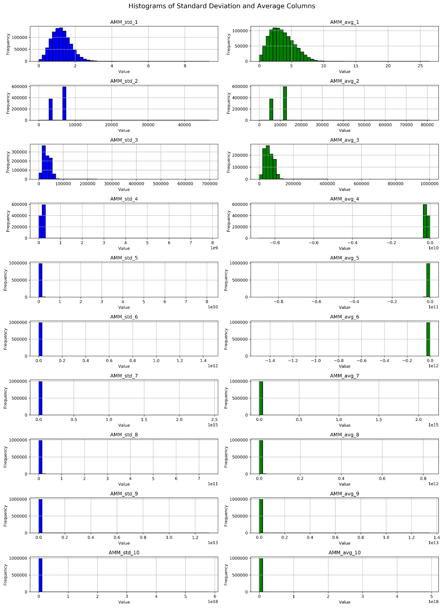
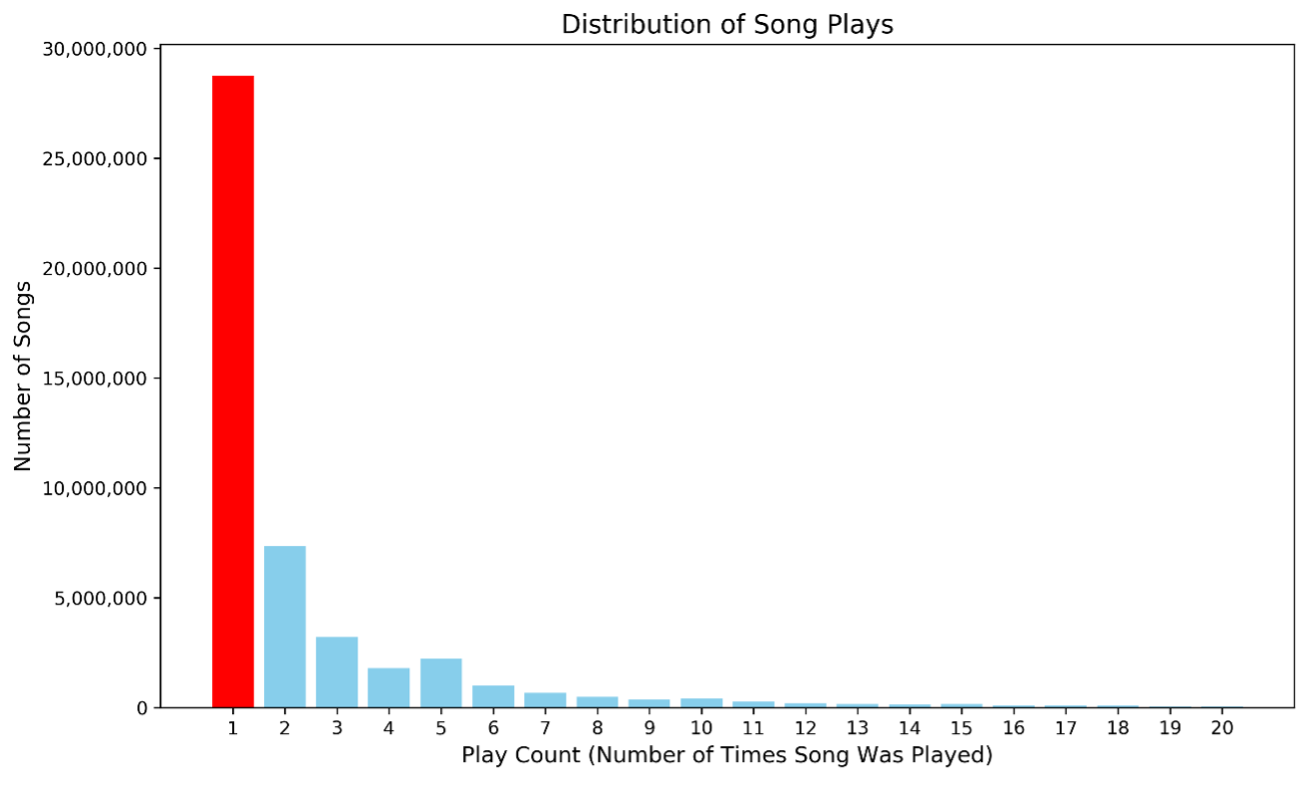
2.2 How features distributed?

In order to know how the features are distributed, the histogram shown the distributed of each feature between mean and standard deviation had been generated (see Appendix C). According to the histogram, it appears that several features have a similar distribution, particularly between standard deviation and average columns. For example, “AMM_std_5” to “AMM_std_10” and “AMM_avg_5” to AMM_avg_10” share the same distribution as it heavily skewed towards the small values with most of data concentrate near zero. On the other hand, the “AMM_std_1”, “AMM_std_3” and “AMM_avg_1”, “AMM_avg_3” show the variation compared to the others but it still appears some skewness. Since features are distributed similarly, they may contribute less to distinguishing between classes lead because it provides redundancy information where features do not add new information for the model. Hence, the model might be struggled to identify the patterns between features and the target variables.

2.3 Features Correlation

To identify any features are correlated, the correlation matrix had been performed to calculate the correlation between each feature. The “VectorAssembler()” used to transform PySpark dataframe into vectors, the feature name now had transform to the vector as 0 to 19, represent 20 feature columns respectively. The Correlation function in “PySpark.ml” was used to perform the correlation matrix (Ayan, 2024). In order to make it easy to read and interpret we transform it into Pandas dataframe and perform a heatmap as below:

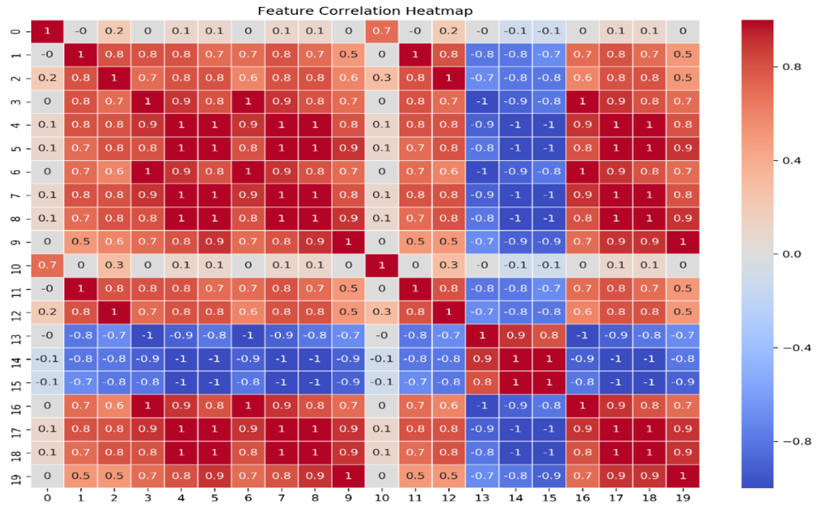
The heatmap shows the pairwise correlations between different features in the MOA dataset. Features with correlations close to 1 (deep red) are strongly positively correlated. For example, feature 5 and feature 19 are strongly correlated (0.9), these features might share the similar patterns. Features with correlations close to -1 (deep blue) are strongly negatively correlated. For example, feature 13 and feature 14 are perfectly negative correlated with a value of -1. Correlations close to 0 indicate a little to no linear relationship between them. Notice that feature 10 only have the high correlation with feature 0 and seem to be very low to no correlation between other features. Moreover, based on the heatmap we can observe that there are many features that perfectly correlated need to be taken into account. In order observe it more detail, we group all the feature pairs that exactly perfect correlated and assign the column names instead of showing the vector number (appendix D). There are 16 features that perfectly correlated with the corelation score of 1 and -1 which is also called the perfect multicollinearity. This might be a potential problem if we include all the features into the model as it will violate the assumption of linear model that independent variables are not perfectly correlated. When independent variables are correlated, the changes in one variable are associated with shifts in another variable, this mean that the stronger the correlation is the more difficult for the model to estimate the relationship between each independent and dependent variable independently (Frost, 2017). According to (Frost,2017), there are some potential solutions to dealing with the multicollinearity such as remove highly correlated features or using Lasso and Ridge regression to shrink the multicollinearity feature less impact to the model. Hence, in this assignment, due to time constraint, we used regularization method to deal with those high correlated features, if we have more time, it also good to deep dive into each feature and explore how it related to genre classification.

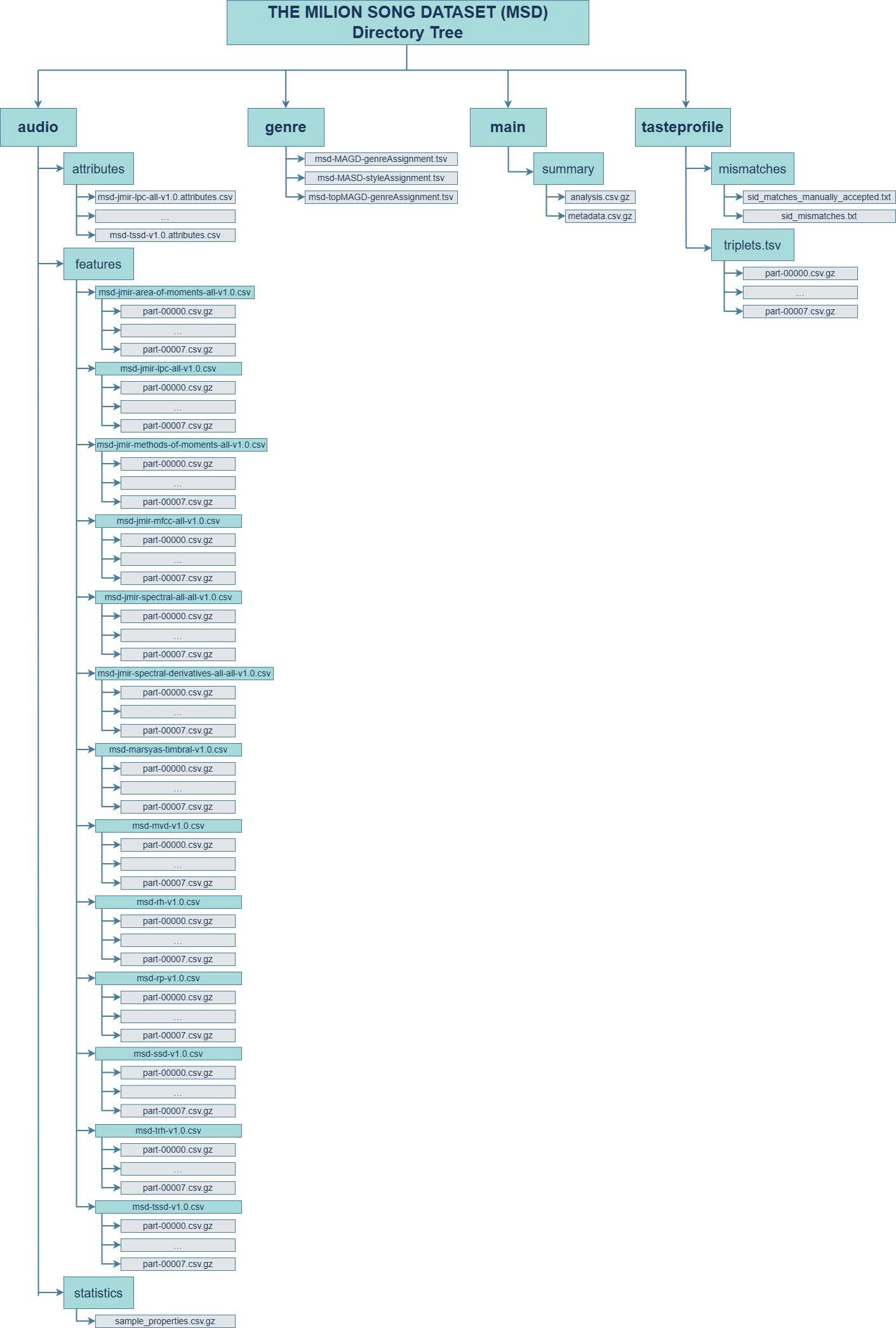
3. Load the MSD Allmusic Genre Dataset (MAGD) & Visualize the distribution of genres

In order to load the MSD Genre dataset, we first define the schema and load the msd-MAGD- genreAssignment.tsv file from HDFS into a Spark DataFrame called MAGD_genre_data. This dataset contains two columns: track_id and the corresponding genre for each song. According to MAGD_genre_data, there are 422,714 tracks with genre information. To visualize the distribution of genres for the tracks that were matched with the audio features, we perform an inner join between MAGD_genre_data and the AOM features dataset using the MSD_TRACKID. This inner join ensures only tracks with both genre and feature data are included. After the join, the resulting dataset, songs_with_genre, is used to visualize the genre distribution and ready for further analysis.

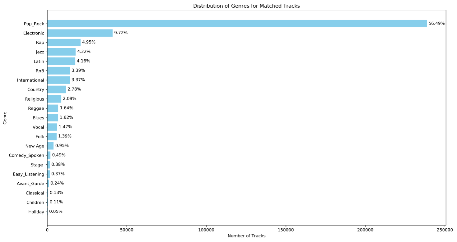
The genre distribution in this dataset reveals a clear imbalance, with Pop_Rock dominating over 56% of the tracks, while smaller genres like Holiday, Children and Classical each make up less than 1%. This uneven distribution can significantly affect the performance of a machine learning model. For example, if we want to predict the Electronic genre, which makes up less than 10% of the total tracks, the model might struggle because it is biased toward predicting dominant genre (Pop_Rock). Even if the model misclassifies most Electronic genre as Pop_Rock, it could still achieve high overall accuracy due to imbalance. However, this would not be useful if our goal is to accurately identify Electronic tracks. In this scenario, the accuracy metric becomes misleading as it does not provide a true measure of the model ability to detect the less common Electronic genre, leading to poor performance in the areas where its matters most.

4. A brief summary of each of algorithms has been chosen

In order to address this classification task, we choose 3 classification algorithms which is Logistic Regression, Random Forest and Gradient Boosted Tree. Logistic Regression (LR) is a linear model, which means it has a relatively simple mathematical structure, leading to fast training speed. It provides coefficients for each feature which represent the strength of and direction of the relationship between feature and target. Due to its high explainability and interpretability, LR is often used as a baseline model. However, it can easily overfit since there are highly correlated features in the AOM dataset as it might give too much weight to redundant information. To address this, regularization techniques such as L1 (Lasso) and L2 (Ridge) will be used to shrink the coefficient of redundant features. Moreover, when perform the regularization, it is sensitive to feature scaling since the penalty will treat features as same scale. According to descriptive statistics, there are huge differences in the range between each feature, it is important to apply scaling method to scale all features to a similar range. Random Forest is an ensemble learning method that builds multiple decision trees and combines them to produce more accurate and stable predictions. It is well suited for handing complex datasets and can handle non linear data and high dimensionality without require data scaling or regularization as it will pick the most important feature to perform a split. However, due to its complexity when building multiple trees, it had slow training speed compared to linear models and also difficult to interpret since it requires some hyperparameter tuning such as number of trees and depth of trees. Gradient Boosted Trees (GBT) is an ensemble learning method that builds a series of decision trees where each subsequent tree corrects the errors of the previous one. This sequential training makes GBT highly accurate and effective at handling both linear and non linear relationships. However, similar to RF, GBT involves many decision trees, making it difficult to understand how the model predicts. It also easy prone to overfitting and huge computational time as it requires many hypermeters tunning.

5. A brief statement of class imbalance and how it affects model.

To convert the genre column into a new binary label the represent Electronic genre and other genre, a new columns called “class” is created with filter if the genre is Electronic than assign the value 1 and otherwise is 0 for other genre using the “F.when” function. By count the number of songs in each class (0 and 1) and calculate the percentage, the class imbalance of a binary model shown as below:

According to table 5, there is a highly imbalanced between Electronic and Non Electronic genre, with approximately 9.67% of the tracks labelled as Electronic and 90.33% are Non Electronic. This imbalance can negatively affect the performance of the classification model. Specifically, the model may become biased toward the majority class, predicting more often due to the larger number of samples. This could create a high accuracy but fail to correctly predict the minority class and could lead to poor performance as our goal is trying to identify the minority Electronic tracks.

6. Explanation of stratify random split and resampling methods

Since there is an extreme class imbalance in the dataset, we apply stratified sampling when performing the train – test split to ensure class balance is preserved. We start by generating a unique ID column, which will allow us to an anti - join later. Next, we create a random column containing random numbers for each row. After that, we generate a new column for row numbers using the window function, evaluated over the window to give row numbers for each class. The window specification is used to partition by our label and order it randomly. Once we have the row numbers, we then define a filter, for label 0 (Electronic) we keep the row if its row number is less than the number of classes 1 (Non – Electronic) rows multiplied by a specific proportion (0.8). Finally, we perform anti join using the ID column generated earlier to obtain the test set, then we drop irrelevant columns. By doing this, we ensure that the class proportion in both training and test sets mirror the original data distribution. The class balance is maintained across both sets, preventing further imbalance. This approach provides consistent class ratios even when running multiple random splits, allowing us to generate reliable precision and recall metrics for test data. The table below show the rows and ratio for training and test. Since our data have a high imbalanced class, before fitting it to the model we want to potentially change this classes proportion in the training data, so the model is more sensitive to our target genre (Electronic). Our goal is trying 4 different types of resampling methods with 3 different models (mentioned above) to determine which yield the best performance. Firstly, we use the oversampling where we are randomly upsample observations of rare classes. The key ideas are keeping the same number of class 0 while upgrade more class 1 which a specific ratio. This might increase the sensitivity without throw away any values. Secondly, instead of creating more class 1 sample, we aim to fewer down class 0 to get a balance proportion between 2 classes. Thirdly, we try to combine both up and down sampling with setting the lower bound and upper bound, this approach seems to be more advance as it changing 2 classes at the same time ensuring both contribute to the class balance. Finally, instead of changing the actual rows, we simply weight the portion of those observations invert to their frequency. For example, in our case we will give the class 1 large weight and underweight for class 0. This allows the training method (e.g SGD) to update the learning rate effectively when it comes across the class 1 and 0. The table below shown the ratio of each resampling methods.

7. Train models and evaluate on test set.

For LR model, we have used 10% from the training dataset to do the 5 - folds cross validation to find the best lambda for regularization. Surprisingly, after 5 folds validation no regularization yield the best AUROC, moreover, we also compare the performance between regularization and non regularization, however, the non regularization yield the best performance over the test set over all sampling methods. After resampling three models had been used to train and evaluate the metrics on the test set as below:

When comparing the different models, AUROC is a suitable as it is based on changing classification thresholds and observing how our true positive and false positive rate trade off each other. Therefore, it is independent on the classification threshold, allows AUROC capturing the overall effective. Based on Table 6, resampling methods significantly improve recall compared to the original models, indicating that these methods help address class imbalance by making the model more sensitive to the minority class. In LR model, while observation reweighting achieves the highest recall, the resampling method provides the highest AUROC. Similarly, for Random Forest, reweighting achieves higher recall, but down sampling yields the best AUROC, making it the most balanced option for this algorithm. Notably, the Gradient Boosted Tree (GBT) model achieves the highest AUROC (0.7175), suggesting it has the strongest ability to distinguish between the Electronic and Non-Electronic classes. Therefore, if the goal is to maximize the ability to distinguish between the two classes, the GBT model with observation reweighting is the best choice due to its highest AUROC.

8. Explanation of how chosen algorithm predict mutiple classes

There are multiple algorithms can be chosen to perform the multiple classification, however, in this assignment, we choose the Logistic Regression (LR) algorithm from “ml.pyspark” to perform the multiple classification for two reasons. First, in spark.ml logistic regression natively supports the multiple classes classification by using multinomial logistic regression with the “family” parameter as it provides a probability across multiple classes (Spark 3.5.3 Documentation, n.d.). Secondly, as mentioned above, LR model have the fast-training speed compared to other models like RF and GBT, due to the time constraint for this assignment, we also choose LR model for time efficiency.

How classes imbalance effect the result?

When transitioning from binary classification to multiclass classification, the class imbalance has changed significantly. In binary case, we only needed to distinguish between two classes with 40, 662 tracks labeled as Electronic, and the rest is grouped into Non Electronic category. However, in the multiclass scenario, it much more diverse distribution across 21 genres with “Pop_Rock” dominating at 237,641 tracks while genre like “Holiday” and “Children” are highly underrepresented with only 200 and 463 tracks respectively. Since our target is trying to have a reasonably balance performance across genres. Therefore, resampling methods was taken into account here since several genre have a very low count which make the model struggle to classify these classes.

9. Stratified random split and resampling method

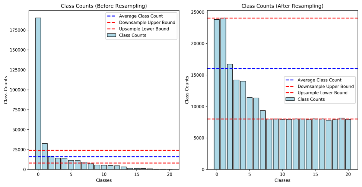
Similar to binary classification, we apply stratified sampling to ensure class balance is preserved. The strategy remains the same as in binary classification, however, instead of splitting two classes, we now split multiple classes while ensuring that each class maintains the same ratio in both the training and test sets. After performing the split, in order to a reasonably balance performance between classes, we perform the resampling method which include up sampling for minority class and down sampling for majority, making it more balanced together. However, we also do not want to make it perfectly balance as in real life there is also a wide distribution between each genre. Therefore, we create the lower bound and upper bound by defined the average class count where we take number of rows divided by the number of classes. For the overrepresentation genres we down sampling it to the upper bound which might less improve model performance but improve the training efficiency and for the underrepresentation genres we want to up sampling to within lower bound.

10. Evaluate multiclass classification performance metric

After resampling the training dataset and make all classes more balanced, we trained Logistic Regression model using multinomial classification to predict all genres. As there are multiple classes, we used the weight metrics such a precision, recall and f1 score to evaluate the performance.

As shown in the table 8, the very low performance metrics across all table, indicate that predicting multiple classes even harder than the binary once especially when there is significant class imbalance. The weight precision 0.454 indicating on overage across all classes 45.4% of the model’s positive predictions were correct. A weighted recall of 0.363 emphasizes only 36.3% the model correctly predicts the actual positive instances. The weighted F1 Score of 0.393 suggests that the model performance in both precision and recall is relatively low, highlighting the trade – off between them. Since precision is calculated as True Positives over predicted positives, when dealing with more than two classes, we weight each class's precision by the proportion of actual positives for that class relative to the total. However, in cases of class imbalance, weighted precision and recall can be heavily biased toward the majority (often negative) class. For example, the model could have 0 precision for a minority class like 'Holiday' but still achieve a high weighted precision due to performing well on the majority class like 'Pop_Rock', similar to how accuracy can be misleading. This means that weighted precision and recall can hide important details about per-class performance. To fully understand the model’s behaviour, it is crucial to examine precision and recall for each class individually.

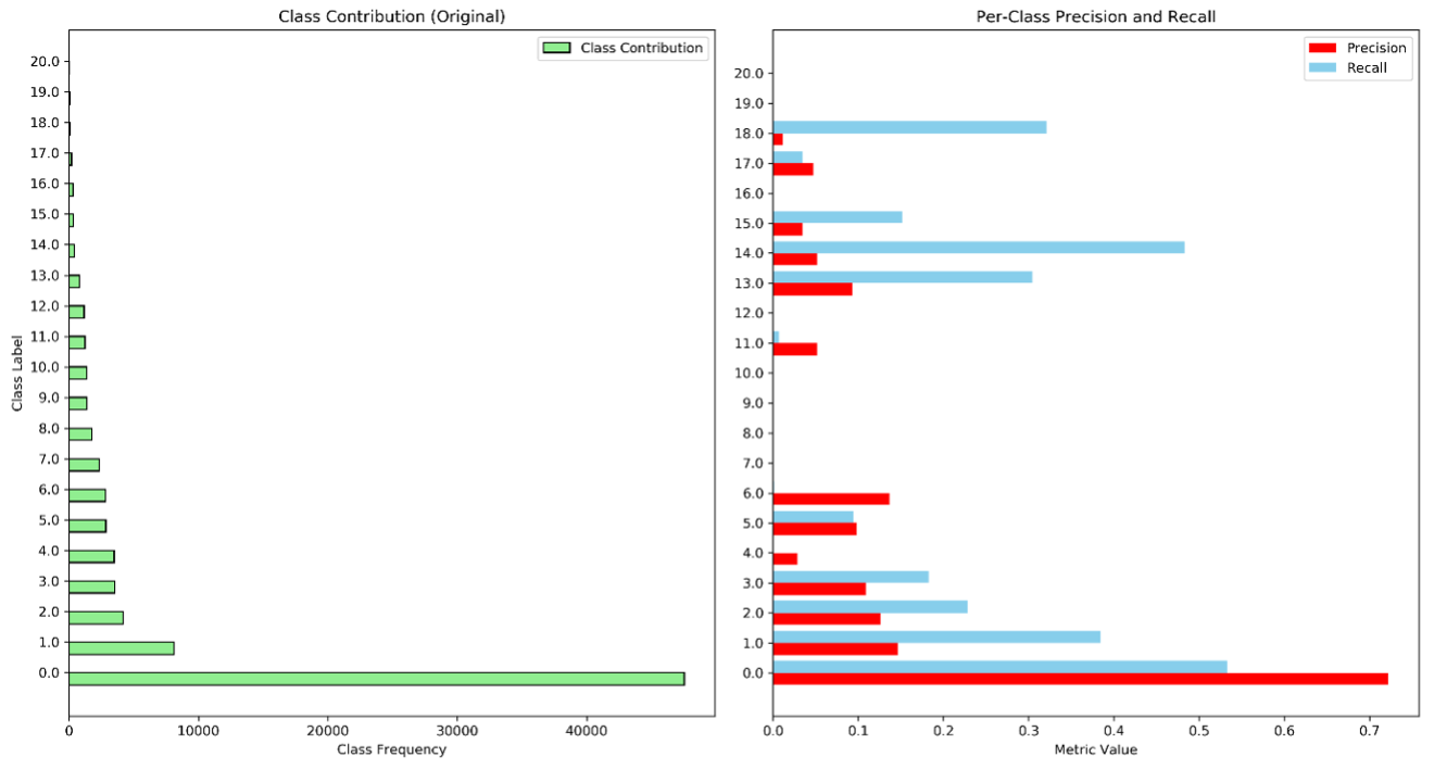
Based on figure 3, there is no surprise that class 0 and 1 have a largest precision and recall across all genre as they have a dominant distribution compared other. Although we already resample the minority classes such as 7,8,9,10,12,19, 20, they also perform not too good in precision and recall, this might because it only create a duplicate value when upsampling which introduce to noise. On the other hand, some of minority class (13,14,15,17,18) have improve the precision and recall after we upsampling it even though it consider as rare classes. As a result, by looking at precision and recall per class and compare it to their original distribution, we can understand how these metrics performed ans why it perform good or bad. Moreover, if we were interested in a particular rare class, we can possibly weight it more in our training.

PART III: SONG RECOMMENDATIONS

I. Explore The Taste Profile Dataset

1. Advantages and disadvantages of repartitioning and caching the dataset

The Taste Profile dataset contains real user-song play counts from undisclosed organisations, it stored in HDFS with 8 “tsv.gz” compressed files, if we load that into Spark it will have 8 partitions, the size of data is 3.3 GB uncompressed, hence each partition would be approximately 412.5 MB when reading the dataset into Spark. By using 2 cores and 3 executor (4 cores in total) we probably do not need to repartition bacause we already got 2 partitions per core which will take a same amount of time as our data have a uniform distribution size. On the other hand, if we want to use more resources, for example try to train different models, we should consider to repartition and cache the result for more efficiency. However, repartition will require a full shuffle as it will re-distribute everything again which take a significant amount of time.

2. Key Statistics for the Taste Profile Dataset

After loading the Taste Profile dataset into HDFS (triplets_data), we used CountDistinct() to identify 384,546 unique songs and 1,019,318 unique users. To determine the number of unique songs played by the most active users, we grouped the data by user_id and counted the distinct songs each user played. The most active user played 4,400 songs, which accounts for 1.14% of the total unique songs. We also generated descriptive statistics for the play_count column to better understand the data distribution. There are 48,373,586 total play counts. The mean play count is approximately 2.87, meaning users typically listened to a song around three times. The standard deviation is 6.44, indicating some variability in play counts. The minimum play count is 1 meaning the smallest play count is a single play, while the maximum play count is 995, showing that some users have listened to a song nearly 1,000 times (table 10). Moreover, by plotting the distribution between number of songs and there play counts (Appendix G), there are 22,084 songs had only played one time and not so many songs play more than 10 times.

3. Distribution of song popularity and user activity

We determine the song popularity by looking at the total play per song as we believe the higher the song play counts, the higher popularity is, hence, this was calculated by grouping the data by “song_id” and count the number of song plays. Similarly to user activity, we consider the more active users, the more songs that they played, therefore, we group the data by “user_id” and aggregate the number songs that users have played then sorted from highest to lowest. Since we only want to understand the distribution of song popularity and user activity, we use the kernel density estimation (KDE) plot to observe the smooth trend, as well as the tails and peaks of the distribution, instead of a histogram. The histogram would be sensitive to bin size, especially in this case, where large bins make interpretation difficult.

Both the User Activity and Song Popularity plots exhibit a heavy right-skewed distribution. This means that the majority of users have listened to only a few unique songs, while a small number of users have listened to a large variety of songs. Similarly, most songs have been played only a few times, while a few songs have been played many times.

II. Train The Collaborative Filtering Model.

1. A brief description of the chosen values for N and M

Since we are going to train colaborative filtering model which used similar users and songs based on their combined play history, hence, songs which have not been played only a few times (N) and users who have only listened to a few songs (M) will not contribute much information to the model. According to (Appendix G), we can observe that most of the songs have been played in the range 1 to 5 which account for 20% of the unique songs. Therefore, we set a minimum threshold where a song must have been played at least 5 times (N = 5), similarly, since we want to working with users who have sufficient interaction history, we decide to defined the most active users is who have listened to at least 10 different songs (M = 10) to included in the cleaned dataset. However, this is just a subjective choice based on what we observed from the data distribution, if would be more reasonable when perform the cross valiadation to choose the optimal M and N if we have time.

2. Numbers of users and songs remain in the dataset

After deciding the thresholds for N and M, we filtered out songs that were played fewer than 5 times and users who listened to fewer than 10 songs using the filter() function. Once these individual filters were applied, we used anti joins to remove both the low-interaction songs and the low-activity users from the original triplets_data dataset. After applying the joins, the number of users and songs remaining in the dataset is displayed as follows.

3. Explanation of why every user in the test set must have at least some user-song plays in training set

The dataset will be split such that the test set includes at least 20% of all song plays. It is essential to guarantee that each user in the test set has corresponding user-song plays in the training set, as the collaborative filtering model relies on user preferences for items such as users, songs and play_count to recommend potential plays or listens of other items. Moreover, numerical indices for users and songs will be required, by using the ‘StringIndexer’ tool to transform user IDs and song IDs from text to numerical format then a pipeline will be used to integrates these steps into a single process and applied to the ‘user_song_play’ dataset. This process generates two additional columns which is ‘user_ID_label’ and ‘song_ID_label’, contain the numerical indices for users and songs. The new dataset will be divided using 'randomSplit' with an 80% training and 20% testing. To verify that users in the test set do not have any interactions in the training set, we conduct a left anti join between the test and training sets. A count of 0 indicates that all users in the test set have interactions with the training set.

4. Train an implicit matrix factorization model using Alternating Least Squares (ALS)

After splitting the dataset, we performed an Alternating Least Squares (ALS) to train the model with the regularization (regParam: 0.01) and 5 maximum iterations.

5. Generate some recommendations, making qualitative comparison

After training the ALS model, we generate the subset of 200 users on the test set to make the qualitative comparison between how the recommendation with the actual users play counts. In order to perform this, we generate the top 10 recommendations for each user and join this with the 200 subset users to find the overlap between each recommendation and their actual play counts. As a result, there are only 3 overlaps between the recommendation and its actual play (Appendix H). This poor performance might come from the intensive outliers, according to figure 6, there are several songs had been played too many times which could be an outliers since it had been playing at the coffee shop or restaurants over times, this could disproportionately influence the model and skew the recommendations toward these overplayed songs and not represent the true user preferences. Therefore, handling with those outliers should be necessary before fitting the model.

6. Compute Ranking Metric on test set and its limitations

In order to evaluate the performance of the recommendation model, we used three ranking metrics as shown below:

Precision @ 10 measures the proportion of relevant songs in the top 10 recommendations. On average, there is 2.86% of the recommendations songs in the top 10 were actual played by users, however, this metric does not take into account the position of the recommendations, it just consider whether it relevant or not. We like the metrics that take into account the position of rank as the top 3 right will be more efficient than the last 3 among 10 recommendations. Therefore, we need the NDCG @ 10 as it not only take into account whether recommended songs is relevant but also the position of the ranking items. However, these metrics were evaluated based on measured historical user interaction data only with no interactions with actual users. Due to the fact that it based on historical user play coutns, it might not be possible to capture the real world context such as current user behavior, user changing preference and real time user 's feedback.

7. Explanation of how we could evaluate the performance of recommendation systems in real world.

Based on the limitation with evaluating ranking metrics in an offline way, an online performance metric will be more advance as we can put our recommendation system in front of the users and exploring the users' behaviors, it much more better compare to the offline metrics as it based on measuring new (live) user interactions with the output of the model. For example, it captures if users click on recommendations or measure some business metric such as KPIs to increase in revenue, user churn assessment which is the rate that users come and leave our platform where we can keep users to continue subscription on our platform if we have the right strategy. Instead of evaluating based on the set of metrics, we calculate the average of daily metrics over time. For example, we use an average click through rate over time to evaluate whether it good or bad. Moreover, the A/B testing can also be used to compare different versions of ranking algorithm to real users at a chosen significant level. As a result, these are some of the methods we can use to assess the ongoing performance of the recommendation model in a production environment as well as to evaluate the real - world system.

PART IV: CONCLUSION

The project explored the Million Song Dataset (MSD) by examining its structure, training binary and multi-class genre classification models, and developing a recommendation system using collaborative filtering (ALS). The AOM features dataset performed poorly in the classification tasks, likely due to its limited ability to distinguish genres and the presence of highly correlated features. With more time, further feature engineering and advanced hyperparameter tuning could improve model performance.

THANK YOU FOR READING!

REFERENCES

1. Ajoodha, R., Klein, R., & Rosman, B. (2015). Single-labelled music genre classification using content-based features. International Conference (PRASA-RobMech). https://doi.org/10.1109/robomech.2015.7359500
2. Fujinaga, I. (1996). Adaptive optical music recognition. Ph.D. dissertation, McGill University.
3. Ayan, D. (2024, February 4). A Guide to Correlation Analysis in PySpark - Davut Ayan. Medium. https://medium.com/@demrahayan/a-guide-to-correlation-analysis-in-pyspark-22824b9a5dda
4. Frost, J. (2017). Multicollinearity in Regression Analysis: Problems, Detection, and Solutions. Statistics by Jim. https://statisticsbyjim.com/regression/multicollinearity-in-regression-analysis/
5. Classification and regression - Spark 3.5.3 Documentation. (n.d.). https://spark.apache.org/docs/latest/ml-classification-regression.html#logistic-regression

APPENDIX

APPENDIX A: MILLION SONG DATASET DIRECTORY TREE

This appendix shows a directory trees structures of the MSD dataset organized in HDFS.

Figure A1: Distribution of AMM standard deviation and average

APPENDIX B: Features Distribution Histogram

This appendix presents how the data had been distributed across features

Figure B1: Distribution of AMM standard deviation and average

APPENDIX C: Perfectly Correlated Feature Pairs

This appendix contains pairs of features that are perfectly correlated, either positively or negatively, as shown in the table.

Figure C1: Feature pairs with perfectly correlated

APPENDIX D: Genres Distribution Across Tracks

This appendix displays the distribution of genres matched with the number of tracks across the dataset.

Figure D1: Feature pairs with perfectly correlated

APPENDIX E: Regularization & Non – Regularization Logistic Regression

This appendix shows the comparison table of difference metrics between Lasso Logistic Regression and Logistic Regression with multiples resampling methods.

Table E.1: Comparison of Logistic Regression (with and without Lasso) Using Different Resampling Methods

APPENDIX F: Distribution of Song Play Counts Across Unique Songs

This appendix shows the distribution of the number of times songs were played, grouped by the number of unique songs.

Figure F.1: Distribution of Song Plays by Play Count

APPENDIX G: Recommendation Qualitative Comparison

This appendix provides a qualitative comparison between recommended songs and actual play counts for different users. Each row corresponds to a unique user and contains their recommended list of items, the items they actual played, and the common elements between these two lists.

Table G1: Comparison of Recommended and Actual Plays with Common Elements