Background
This assignment focuses on analysing the Global Historical Climatology Network (GHCN) daily dataset using Apache Spark. The GHCN dataset contains global climate observations, making it vital for understanding long-term climate patterns. The initial task involves understanding the dataset structure and loading it into Spark for efficient processing. Key data processing steps include inspecting variables and merging relevant metadata to enrich station data. In the analysis phase, we explore trends in climate variables like temperature and precipitation, calculate distance between two stations, generate descriptive statistics, and conduct time series analysis to detect seasonal and long-term patterns. Additionally, we summarize the data by regions and time periods to uncover larger climate trends, with a focus on stations in New Zealand. Spark's distributed computing capabilities enable efficient handling of large datasets throughout this process.
PART I: PROCESSING
I. Explore the daily, stations, states, countries, and inventory data in HDFS
1. How is the data structure?
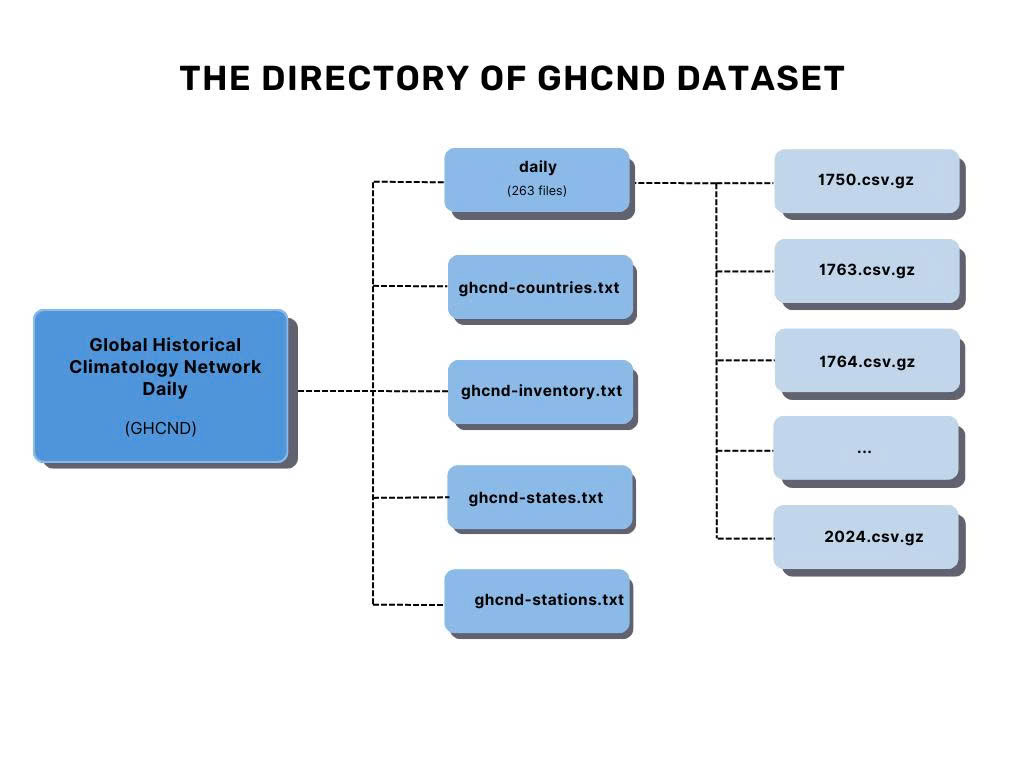
The GHCND dataset is stored in Hadoop Distributed File System (HDFS) and is organized into a main directory containing daily climate observation with 263 compressed CSV files. The first year in daily dataset is 1750 following the 13 years gap and until 1763 to 2024. Alongside the daily data, the directory includes metadata files such as ghcnd-countries.txt, ghcnd-inventory.txt, ghcnd-states.txt, and ghcnd-stations.txt, which provide essential information about the countries, weather stations, and recorded variables.
2. How does the size of the data changes?
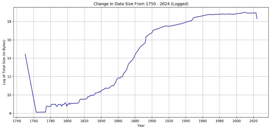
The chart shows the change in data size from 1750 to 2024. By taking the log we can observed there is the gap between 1750 to 1763 indicate the missing data between those years which hard to see in the original scale. From 1763 to 1880, the data size grows steadily and gradually. However, starting in 1900s, there is a sharp increase. After 1950, the growth becomes more stable toward the end of series.
3. What is the total size of all of the data, and how much of that is daily?
The total size of the GHCND data is 12.5 GB, representing the actual amount of data stored, and 99.8 GB, which includes replication across the HDFS. The daily data specifically comprises 12.4 GB (actual size) and 99.5 GB (HDFS size). Since each dataset have several different sizes of unit such as (GB, KB, MB), in order to explore how the size of other datasets compare to daily dataset, we have to convert it into the same consistent unit. According to the table 1, the daily dataset dominates the data volume with 13002342.4 KB, accounting for 99.66% of the total. In comparison, the inventory dataset, which is 33,996 (KB) represents only 0.26% of the total. The stations dataset has 10,752.0 KB (0.08%), while the countries and states datasets are minor in size, with 3.6 KB and 1.1 KB, respectively. In conclusion, the daily dataset is vastly larger than the others combined.
| Datasets | Actual Size | Replicate Size | Actual Size in KB | Percentage Total (%) |
|---|---|---|---|---|
| Daily | 12.4 GB | 99.5 GB | 13002342.4 | 99.656985 |
| Countries | 3.6 KB | 28.6 KB | 3.6 | 0.000028 |
| Inventory | 33.2 MB | 265.4 MB | 33996.8 | 0.26057 |
| States | 1.1 KB | 8.5 KB | 1.1 | 0.000008 |
| Stations | 10.5 MB | 84.0 MB | 10752 | 0.082409 |
II. Apply the schema to each dataset
1. Define the schema for daily dataset
The schema for the daily dataset follows the format recommended in the README file, with data types selected to match each column's data. StringType is used for character data, while IntegerType is applied to numeric fields like "Value." The "Date" variable is formatted as StringType due to null values, and "Observation_Time" is defined as TimestampType to handle the HHMM (hour-minute) format. The nullable in Station_ID column is set to be false since we do not expect this field have the null values.
2. Load 1000 first rows of the 2023 daily dataset
After changing the “DATE” variable into the “StringType” the 1000 rows of 2023 daily dataset had been loaded successfully. The table contains the final schema for daily dataset are shown below:
| Data Type | Variable Names |
|---|---|
| String | Station_ID, DATE, Element, Measurement_Flag, Quality_Flag, Source_Flag |
| Integer | VALUE |
| Timestamp | Observation_Time |
3. Load each stations, states, countries and inventory dataset
Since the GHCND metadata is in a fixed-width format, we use the substring function in the PySpark API to extract specific data from string columns based on their positions within the fixed-width structure (PySpark 3.1.1 Documentation, n.d.). Additionally, loading fixed-width files often introduces extra spaces that can cause formatting issues. The trim function is crucial in this context as it removes any leading or trailing spaces from the extracted strings (pyspark.sql.functions.trim – PySpark 3.5.2 Documentation, n.d.). Therefore, both substring and trim are essential for parsing and correctly formatting fixed-width text data. After parsing the data and correctly assigning it to the appropriate columns, each variable was then converted to the correct data type. The table below shows the total number of rows for each dataset along with the variable names and their respective data types.
| Metadata | Row Counts | Data Type | Variable Names |
|---|---|---|---|
| States | 74 | String | State_Name |
| Countries | 219 | String | code_country, Country_Name |
| Stations | 127,994 | String | Station_ID, State_Code, Station_Name, GSN_Flag, HCN_CRC_Flag, WMO_ID |
| Double | Latitude, Longitude, Elevation | ||
| Inventory | 756,342 | String | Station_ID, Element |
| Double | Latitude, Longitude | ||
| Integer | First_Year, Last_Year |
4. Checking overlap between stations and inventory
To determine if there are any stations in the inventory table that are not present in the stations table, we use a left anti join with the station_id as the key. The left anti join selects only the rows from the left table (inventory) that do not have corresponding matches in the right (stations) table (Nelamali, 2024). After performing this join, the result was counted to identify how many such stations exist. The count was 0, indicating that all stations inventory table are also present in the stations table.
PART II: EXPLORE STATIONS METADATA FILE
Enriching Station
1. Combining relavant information
To explore the station tables in more detail, the stations data was enriched by joining it with both the countries and states data. First, the country code was extracted from each station ID using the substring function, and this was stored in a new column named "country code" with the withColumn method. This new column was used to perform a LEFT JOIN between the stations and countries data. Similarly, the stations data was joined with the states data using the "State_Code" column for more detailed information. The use of LEFT JOINs ensured that all stations remained in the dataset, even if corresponding country or state information was missing, allowing for comprehensive analysis without losing any station records. These joins transformed the station dataset into a more informative one, enriched with geographic metadata valuable for location-based analysis.
2. The first & last year each station active
To determine the first and last years each station was active and collected any element, the analysis began by grouping the inventory data by “station_id” and using aggregation functions to find the minimum and maximum years each station was active, the resulting then stored in “station_year” table which provided a clear timeline of when each station was operational. For further information, the length of time that each station active calculated by subtracting the First_Year from the Last_Year and adding one year to account for the inclusive range. In overall, there are 2701 stations were active for only 1 year represent the shortest operational and 64 stations were active for the maximum period of 275 represent for the longest operational. In average, stations were active for approximately 35 years.
3. Count of Different, Core, and "Other" Elements Collected by Each Station
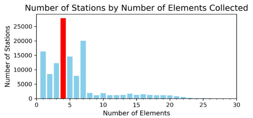
According to the “README” file, there are five core elements which is PRCP (Precipitation), SNOW(Snowfall), SNWD (Snow depth), TMAX (maximum temperature), TMIN (minimum temperature). To count the number of different elements that each station had collected, the method began by defining the core elements list and using the “withColumn” to create the two new columns which identifies whether an element is a core element (1) or not (0). Next, the data was aggregated by station_id to calculate the number of unique elements collected by each station using the count distinct and sum function. Finally, the result had been joined with the station_year table above to ensure all relevant information is captured and was stored under the “element_counts” dataset. As a result, there are 2 stations that collect 70 elements, which is considered the highest number of unique elements that any station can collect. In contrast, there are 16,390 stations that collect only 1 element, considered the lowest. Most stations collect between 1 to 10 elements, with 4 being the most common number of elements collected, as indicated by the peak in the distribution (Figure 3).
4. Stations collected all five core elements
There are 20,482 stations that collected all five core elements, this result by filtering element_counts table include only those stations where the core elements count equal 5.
5. Stations collected only precipitation (PRCP)
To determine the number of stations collected only precipitation the “sql.collect_set” had been used to collect the unique elements each stations had recorded the filtered only those set contained exactly precipitation element. As the result, there are 16,308 stations that collect only precipitation (PRCP).
6. Schema of Enriched Station
The element_counts table then joined with the station data based on the station_id which create a new dataframe name enriched_stations (see schema table below). Since Parquet’s columnar storage structure enables faster read operations and significantly reduces the amount of data read from disk, which is ideal for analytical queries. Additionally, Parquet enforces a schema, ensuring data consistency across operations and preventing structural inconsistencies issues since no need to redefine the schema (Kushwaha, 2024). As a result, the enriched_stations had been saved as Parquet file format for later analysis.
| Data Type | Variable Names |
|---|---|
| String |
Station_ID, Station_Name, GSN_Flag, HCN_CRN_Flag, WMO_ID, COUNTRY_CODE, Country_Name, State_Code, State_Name |
| Double | Latitude, Longitude, Elevation |
| Integer |
First_Year, Last_Year, Total_Years_Active, Total_Unique_Elements, Core_Element_Count, Other_Element_Count, Total_Unique_Elements |
II. Comparison stations with daily dataset
1. Stations in subset of daily thar are not in stations
Since the entire daily data is large, it might waste a huge number of resources if checking all the missing stations all over the data. Therefore, to check the missing stations in daily, 1000 subset rows in daily data had been used to validate. A left anti join was performed between this subset and the stations dataset to identify any stations present in the daily subset but not in the station’s dataset. This approach returns only the rows from the daily subset where no corresponding match is found in stations. The result showed zero unmatched stations, indicating a complete match between the two datasets for this subset.
2. The expensive of a left join & alternative approach
The daily dataset is extremely large, with over 3 billion rows, while the enriched station is small which only contains 127,994 rows. In a left join, every row from daily dataset must be checked against the enriched stations, which means that the join operation needs to handle a massive volume of data. Spark often needs to shuffle data across the network to perform joins. Since the daily dataset is large, this shuffling can become a major bottleneck. A more efficient way to perform this operation would be to use a broadcast join. As the enriched stations dataset is small, it can be broadcasted to all worker nodes in the cluster (Necati, n.d.). By broadcasting enriched stations, each executor has a local copy of the smaller dataset, allowing for a fast and efficient join with the large daily dataset (Singh, n.d.). This approach eliminates the need for shuffling the large daily dataset across the network which save computation time, making the operation much more scalable.
3. Number of stations in daily that are not in stations
To efficiently count the number of stations in the entire daily dataset that are not in the station dataset, a broadcast join was utilized, follow by performing an anti-join to identify any stations in the daily dataset does not present in the station’s dataset. The result showed that there are no missing stations in the daily dataset, as the count returned zero.
PART III: EXPLORING THE DAILY CLIMATE SUMMARIES
I. Understand the structure and format of daily dataset
1. Default block size in HDFS & Number of block required for the daily
| 2023 | 2024 | ||
|---|---|---|---|
| Default block size (MB) | 128 | ||
| File Size (MB) | 168.40 | 88.8 | |
| Number of blocks | 2 | 1 | |
| Size per block (MB) | Block 1 | Block 2 | Block 1 |
| 128 | 34.1 | 88.8 | |
The default block size in HDFS is 134,217,728 bytes which equivalent to 128 MB (1 MB = 1,048,576 bytes). For the daily climate summary file in 2024, which is 88,831,735 bytes (88.8 MB) and 8 replications, only one block is required because the file size is smaller than the default block size. For the 2023 climate summary file, which is 168,357,302 bytes (168.4 MB) and 8 replication, two blocks are required
The first block is 134,217,728 bytes (128 MB), and the second block is 34,139,574 bytes (34.1 MB). The first block is filled to the default block size limit, and the remaining data is stored in the second block (table 5). Since all the replicates can be found in HDFS (Live_repl = 8), therefore all the files are healthy.
2. Load and count the number of observation in 2023 & 2024
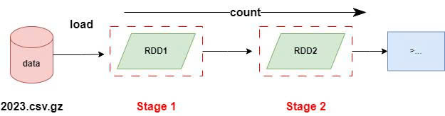
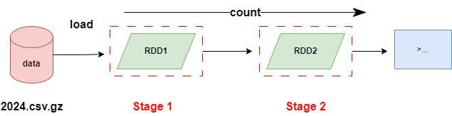
In Spark, a job is triggered by an action. In this scenario, there are two jobs: one for loading and counting the 2023 dataset, which contains 37,867,272 observations, and another for the 2024 dataset, which has 19,720,790 observations. Each job is divided into stages based on shuffle operations or transformations that require moving data across partitions. Since reading the data and counting the data still involves a reduce operation under the hood otherwise, we cannot get the total line count on one worker node to send that output to the master node, therefore, each job will consist of two stages (Figure 4). The number of tasks within each stage depends on the number of partitions in the dataset. As both the 2023 and 2024 datasets are compressed, there is only one partition in each file, so the data reading and counting operations are completed in a single task per stage. As a result, there are two jobs, each with two stages, totalling four stages and four tasks executed across both jobs.
3. Number of Files & Blocks Determines Task Count for Observation Counting
The number of tasks does not always correspond to the number of blocks in each input. For example, the 2023 dataset was stored across 2 HDFS blocks (128 MB and 34.1 MB). Since the block size is configured to be 128 MB in HDFS, this data typically split into 2 blocks and will have 2 tasks if each task processes one block. However, due to the file being compressed with Gzip, the situation is different, when Spark encounters a Gzip compressed file, it must be read the entire file as a single unit without parallelizing the read operation across blocks otherwise it would lead to corrupted chunks, because Gzip does not support splitting regardless of how many HDFS blocks it spans (Apache Spark and Data Compression, n.d). As a result, Spark creating only 1 task to process the entire file.
4. Load and Count Observations from 2014 - 2023: Task Execution and Input Partitioning
To load and count the total number of observations for the years 2014 to 2023 inclusively, a glob pattern was applied in the file path argument of the “read.csv()” function in Spark. Glob patterns are a type of wildcard syntax that allows specifying multiple files with a single expression (Select Files Using a Pattern Match, n.d.). In this case, the pattern {2014 to 2023} was used to match files corresponding to each year within the specified range.
| Read and Count Number Observations 2014 - 2023 | ||
|---|---|---|
| Number of jobs | 1 | |
| Stages | 2 | |
| Stages ID | Stage 10 | Stage 11 |
| Tasks per Stage | 10 | 1 |
| Input Sizes | 1581.1 MiB | |
| Total Tasks Count | 11 | |
This operation involves only one job, which is loading and counting 370,803,270 number of observations in the years between 2014 to 2023. For this job, there are 2 stages, which are defined as Stage 10 and Stage 11 in Table 6. The first stage processed an input size of 1581.1 MiB, which was split into 10 tasks. The input data from the years 2014 to 2023 was divided into 10 partitions, with each partition being processed by a separate task. This partitioning occurred because the input files were compressed, and Spark typically treats as non-splitable partition (Achyuta, 2023), leading to one task per file. In this case, there were 10 compressed files one for each year, resulting in 10 partitions and, consequently, 10 tasks. The second stage performed the final count operation, which required only 1 task since the data had already been aggregated and did not require further partitioning. In conclusion, there is 1 job and 2 stages, which total 11 tasks: Stage 10 has 10 tasks one for each year of data, and Stage 11 has only 1 task for the final aggregation.
5. A summary of how to increase tasks run parallel
According to the 2023 and 2024 daily dataset, the file is stored in HDFS as a Gzip file, which cannot be split, Spark must read the entire file in a single task without parallel processing. By changing the file format to one that supports splitting, such as CSV or plain text, Spark can divide the file into multiple partitions and process them in parallel. This change would reduce the processing time when loading and counting the data.
Since parallelism is limited when working with Gzip files in Spark due to the fact that each Gzip file is processed as a single partition, optimization can be achieved by processing as many Gzip files concurrently as possible. By using 4 executors and 2 cores per executor, we have a total of 8 cores available for task execution, allowing up to 8 tasks to run in parallel. Spark can thus process 8 Gzip files concurrently (as shown in Table 8), with the remaining 2 tasks processed afterward. The table below demonstrates that increasing the number of executors to 4 and utilizing all available cores can significantly reduce the execution time by 3.56 times, ensuring efficient use of resources.
| Job | Read and count the observations in 2014 - 2023 (inclusive) | |||
|---|---|---|---|---|
| 2 executors, 1 executor per core | 4 executors, 2 executors per core | |||
| Stages | First Stage | Second Stage | First Stage | Second Stage |
| Number of tasks | 10 | 1 | 10 | 1 |
| Tasks run parallel | 2 | 1 | 8 | 1 |
| Executive time (second) | 57s | 16s | ||
PART IV: Analysis
I. Overview of Stations Before Analysing Dailiy Climate Summaries
1. The number of stations in total, stations were active in 2024, stations in more than one network.
The analysis began by loading the enriched stations dataset from Parquet and make a simple count distinct operation to determine the total number of stations which result in 127,994. Next, a filter operation was applied to find out stations active in 2024, resulting that 35,616 stations were active. Furthermore, to analyse the distribution of stations across specific climatology networks, the dataset was filtered based on the “GSN_Flag”, ” HCN_CRN_Flag”, and “HCN_CRN_Flag” columns. The result showed the presence of 991 stations in GCOS Surface Network (GSN), 1,218 in the US Historical Climatology Network (HCN), and 234 in the US Climate Reference Network (CRN). By filtering the stations with the GSN_Flag equal to 'GSN' and similarly filtering those with HCN_CRN_Flag, we count how many stations satisfy these conditions. As a result, there are 15 stations that belong to more than one network.
2. Number of stations are there in the Southern Hemisphere & Territories of USA arounf the world.
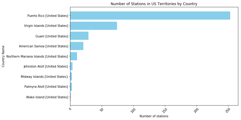
To find out how many stations are in the Southern Hemisphere, we can filter the data frame based on the latitude of the stations. Since the negative latitudes represent Southern Hemisphere (Latitude/Longitude Format | PacIOOS, 2018). Therefore, we can filter stations that have the negative latitude. As a result, there are 25,357 stations are located in the Southern Hemisphere. To determine the number of weather stations located in the territories of the United States around the world, excluding the mainland U.S., the dataset was filtered to include only those records where the country name contains "United States" but the country code is not 'US'. This filtering method ensured that only stations in U.S. territories were counted, excluding any stations in the continental United States. The result of this analysis revealed that there are 399 weather stations located in U.S territories around the world with the highest is Puerto Rico follow by Virgin Islands and Guam (see Appendix B).
3. Count the total number of stations in each country & state
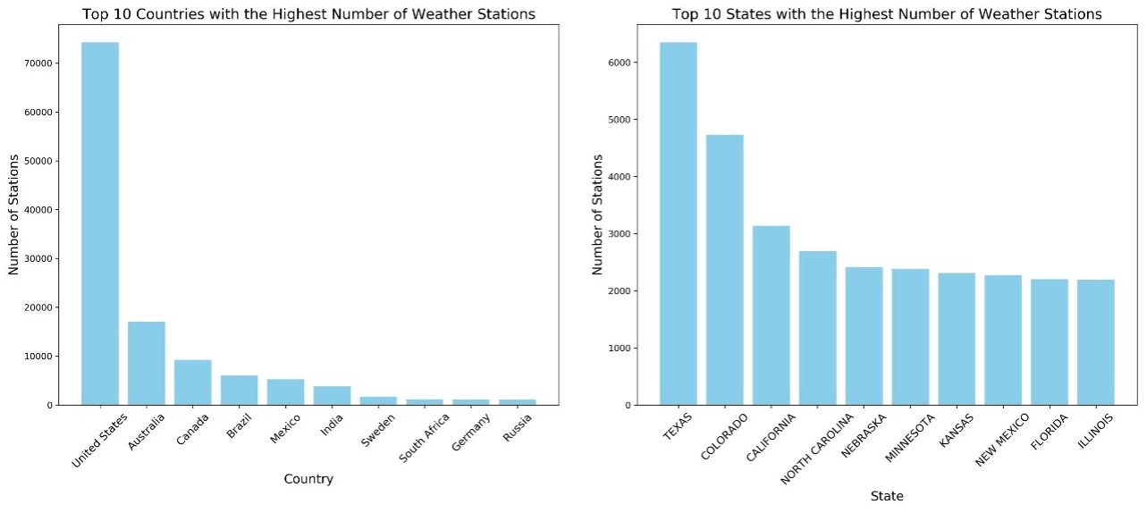
The process starts by grouping the stations data by country code and counting the number of stations in each country using the group by and aggregate functions. The result is then joined with a dataset of countries, which is loaded from HDFS. This enriches the station data with country names, providing a clear view of the number of stations in each country. Similarly, the same method is applied to the states within the countries, offering detailed insights into the distribution of stations at the state level, these results was then saved to hdfs directory. According to Figure 5, the United States has the highest number of stations, followed by Australia and Canada. This is consistent with the observation that the top three states with the highest number of stations Texas, Colorado, and California are also located in the United States.
II. Geographical Distance Between 2 Stations
1. Haversine formula
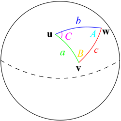
Since Euclidean distance assumes two points lie on a flat surface (Wikipedia, 2024), it is not accurate for real-world distances. The Haversine formula, on the other hand, calculates the shortest distance between two points on the Earth's surface using latitude and longitude, making it a more precise method for measuring geographical distances. It accounts for the Earth's spherical shape by converting these coordinates into radians and calculating the value square of half the chord length between the points. The central angle between the two points is then computed based on this squared of half the chord length. This angle is multiplied by the Earth's radius to find the distance, ensuring an accurate measurement on a curved surface (Bielski, 2019; Prasetya et al., 2020). The output is the shortest distance along the Earth's surface, accurately reflecting the spherical nature of the Earth. The Haversine formula shown below for better illustrate and has been generated using Python for stations distance calculation.
$$a = \sin^2\left(\frac{\Delta\varphi}{2}\right) + \cos(\varphi_1) \cdot \cos(\varphi_2) \cdot \sin^2\left(\frac{\Delta\lambda}{2}\right)$$
$$c = 2 \cdot \mathrm{atan2}\left(\sqrt{a}, \sqrt{1-a}\right)$$
$$d = R \cdot c$$
Where:
\(\varphi\) = latitude
\(\lambda\) = longitude
\(R\) = Earth radius (6371 km)
\(a\) = square of half the chord length between the points
\(c\) = central angle
\(d\) = distance between points
Figure 6. The Haversine formula
2. Validate the Haversine Function
For validating, we used the small subset of stations in United States named and performing cross join to create a pair of stations. As the distance from station to itself is zero, the filter method was then applied to filter out the stations to itself. In conclusion, the Haversine function was then applied to obtain the distance between each station (see Appendix A).
Geographically closest station in New Zealand: To find the geographically closest stations in New Zealand, we filtered the dataset to include only New Zealand stations and applied the Haversine function to calculate the distance between each pair. We then sorted the results by distance to identify the closest pair, which were Wellington Aero AWS and Paraparaumu AWS, with a distance of 52.09 kilometre (table 8).
| Station ID 1 | Station Name 1 | Latitude 1 | Longitude 1 | Station ID 2 | Station Name 2 | Latitude 2 | Longitude 2 | Distance KM |
|---|---|---|---|---|---|---|---|---|
| NZM00093439 | WELLINGTON AERO AWS | -41.333 | 174.8 | NZ000093417 | PARAPARAUMU AWS | -40.9 | 174.983 | 52.09 |
III. Daily data in detail
1. Number of rows and observations in daily and 5 core elements
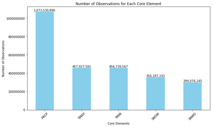
The daily dataset has 3,119,374,043 rows. By applied the filtered to include only the observations corresponding to the five core elements (PRCP, SNOW, SNWD, TMAX, and TMIN) using the filter method, the subset of data containing these elements was grouped by the Element column, and the number of observations for each element was counted using the group by and count functions. As a result, the element with the most observation is Precipitation (PRCP) with 1,073,530,896 observations followed by TMAX and TMIN element (see Appendix C).
2. A number of observations of TMAX have no TMIN
To determine the number of observations where TMAX does not have a corresponding TMIN, the dataset was first filtered to focus exclusively on temperature elements, specifically TMAX and TMIN. The data was then grouped by Station_ID and DATE, and the collect set function was used to aggregate the unique elements observed for each group. Since the daily dataset is large, this approach was chosen to reduce computationally expensive because it reduces data movement across the partitions. The array contains function was applied to filter these grouped records, checking for the presence of TMAX and the absence of TMIN. The final count were 10,567,304 observations where TMAX was recorded without a corresponding TMIN account for only 2.31% in total. These observations were contributed by 28,716 unique stations.
PART V: TIME SERIES & GEOSPATIAL VISUALIZATIONS DAILY CLIMATE
I. Time Series of TMIN anf TMAX across New Zealand
1. Summary of observations and time period covered
To determine the number of observations and the number of years covered, the dataset was filtered to obtain all observations of TMIN (minimum temperature) and TMAX (maximum temperature) for all stations in New Zealand. This was done by extracting the first two characters of the “station id”, which represent for the country code. The filtered dataset contains 487,760 observations of TMIN and TMAX, covering a period of 85 years. The result was then saved to the HDFS directory as CSV format for further visualization.
2. Time series of TMIN & TMAX for each station in New Zealand
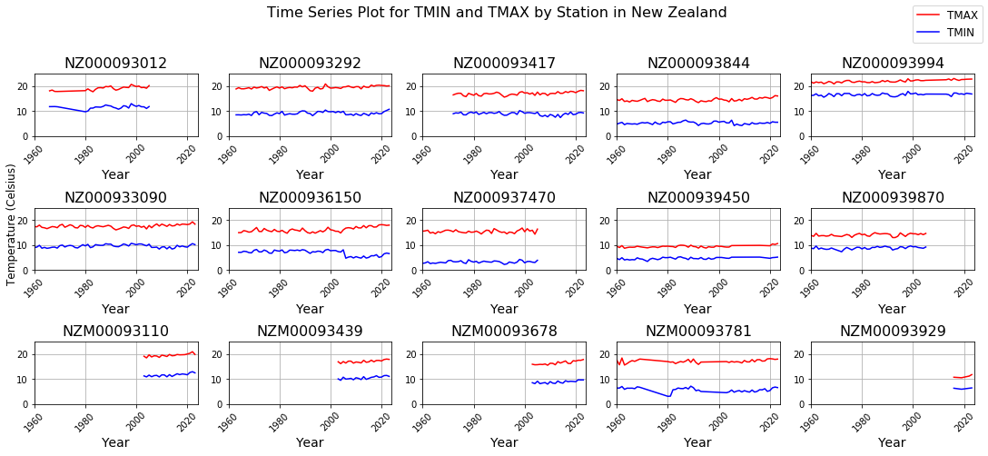
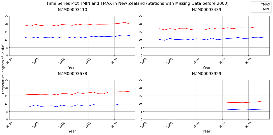
The new folder was created to store the part files containing TMIN and TMAX data for stations across New Zealand, which were copied from HDFS to the local machine for easier access. All of the CSV files were loaded and concatenated into a single data frame. The data was then filtered to retain only the relevant columns to facilitate more efficient manipulate. Since some stations have only collect a few records for whole year it will be not accurately represent the full annual cycle. Therefore, exclude these years ensures the time series reflects full annual data, making comparisons across years more consistent and reliable between stations. As the value represent in tenths of Celsius degree for each station, for easy human read the value had been converted to standard degrees Celsius. Since data smoothing is essentially the process of averaging data points in a time series (Dancker, 2022), to account for short-term fluctuations and emphasize long-term trends, a yearly average was applied for calculate the TMAX and TMIN values for each year. This method effectively reduces noise, making the underlying trends more visible in the visualizations. A series of subplots were generated for 15 stations, displaying the time series of TMAX and TMIN values across New Zealand (see Appendix D). The y-axis was kept consistent across all plots to allow for better comparison between stations. As a result, it was observed that four stations had missing data prior to the year 2000 consider as gaps in data, as shown in the Figure 6 below:
3. A visualization of the average TMIN and TMAX for all New Zealand
To visualize the average minimum and maximum temperature for entire New Zealand, the data was then group by year and calculated the average TMIN and TMAX for the entire country as below:
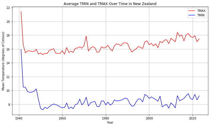
The plot shows the average maximum (TMAX) and minimum (TMIN) temperatures in New Zealand from 1940 to 2024. The initial drop in temperature may be due to early data coming from only a few warmer stations. As more stations, including those from cooler regions, were added over time, the average temperature dropped. Following this drop, the plot shows fluctuations. From 1960 there is a gradual rise in temperatures over time, particularly reflecting the warming trend.
II. Precipitation Observations Around the World
1. The average rainfall in each year for each country
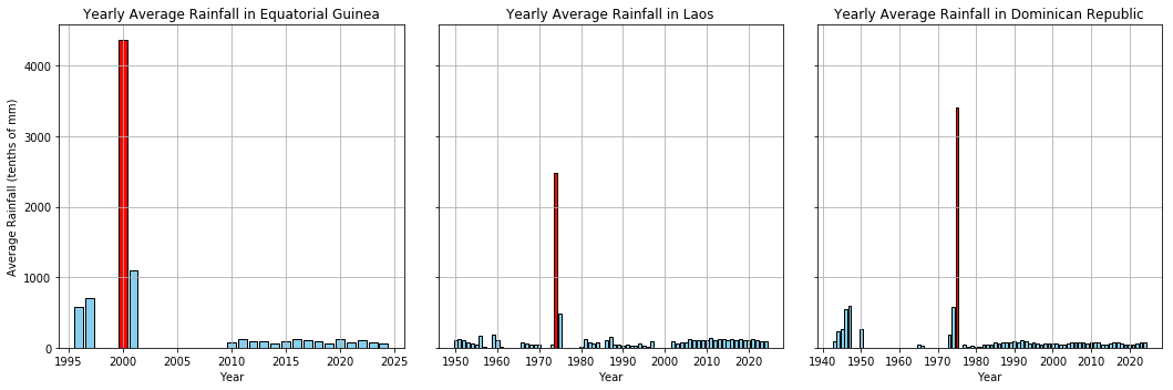
The daily dataset was filtered to retain only precipitation (PRCP) records with values greater than or equal to 0, as rainfall cannot be negative and ensuring that both rainy and dry periods are considered. The columns "Year" and "Country_Code" were added using the substring function, and the average rainfall for each year in each country was calculated, including days with no rainfall (value of 0), this allows for fair comparisons between countries with different rainfall patterns (e.g., tropical vs. arid regions). A broadcast join was then used to merge the result with the country table to retrieve the country names using the country code. The analysis shows that Equatorial Guinea had the highest average rainfall, with 4361 tenths of mm in 2000. However, this result is not sensible because the station in Equatorial Guinea recorded only one data point in 2000, meaning the annual average is based on a single day's rainfall and is therefore not representative of the entire year.
2. Descriptive statistics for the average rainfall
| Summary | Average Rainfall |
|---|---|
| Count | 17384 |
| Mean | 41.82 |
| Std dev | 84.49 |
| Min | 0.0 |
| Max | 4361.0 |
The descriptive statistics of average rainfall were generated using the Spark describe function, covering 17,384 entries. Since days with no rainfall were included in the analysis, the overall average rainfall is lower, with a mean of 41.82 tenths of mm. The minimum value of 0 reflects the days with no rainfall, which skews the average downward. The maximum value of 4361.0 tenths of mm is highly misleading, as it comes from a station that recorded only one day of rainfall for an entire year. This might be an extreme outlier that does not reflect typical rainfall patterns. The standard deviation of 84.49 tenths of mm indicates a high level of variability in the data, further exaggerated by the inclusion of both dry days and extreme outliers. Therefore, the statistics, particularly the mean and maximum, are not fully sensible. Given the extreme variability observed in the descriptive statistics, it would be interesting to look at several extremely high average rainfall values. Based on the yearly average rainfall data, there are three countries have the extremely high value which is Equatorial Guinea (4361 tenths of mm), Dominican Republic (3414 tenths of mm) and Laos (2480.5). These high value abnormal compare to there previous recorded (see Appendix E), which might because that these stations only recorded the value as a whole year rainfall or maybe it just recorded only the rainfall day, where should be take into account by investigation how the data was collected for these stations. As a result, several stations might have different collected method and not collected equally in each year, which lead to the fact that calculate the yearly average rainfall based on the number of observations might not be a concise approach.
3. Plot the average rainfall in 2023 for each country
To address this issue, the total rainfall and the number of recorded days for each station in 2023 are first calculated, assuming that stations without any records during certain periods represent dry periods. The yearly average rainfall is then computed by dividing its total rainfall by the actual number of days it recorded. Since this calculation is weighted by the number of days each station recorded, stations with more data contribute more significantly to the final country average, the approach minimizes the influence of outliers into the overall average rainfall. As a result, the approach produces a more balanced and concise representation of rainfall across all stations within a country. The result was then converted to millimetre (mm) for easy interpret and saved to local for visualizing.
Since Geopandas library does not support two characters country codes, country names were used for mapping. Several bracketed text in country names (e.g., U.S. territories) was removed to maintain consistency. To match country names between datasets, three methods were employed. First, regular expressions were used to match the first four characters of country names. Second, the FuzzyWuzzy library, using a 90% similarity threshold, matched names based on Levenshtein distance to calculate differences between sequences (FuzzyWuzzy, 2020). A combining column was created, based on whether the name was found by these two approaches. Finally, manual adjustments were made for countries that could not be matched by either method. The dataset was then merged with the Geopandas world dataset to plot global rainfall (Figure 16). As a result, some small countries and islands (e.g., Singapore, Maldives) do not appear in the Geopandas world dataset, which is why 31 countries could not be matched.
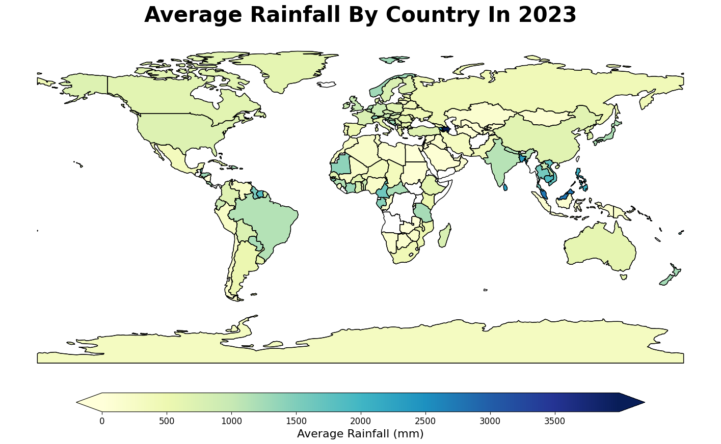
The rainfall map shows the average rainfall across countries in 2023. Most countries fall within moderate rainfall ranges, aligning with the World Bank’s annual precipitation dataset (Average Annual Precipitation, 2024), as indicated by lighter shades of green and yellow. White areas represent countries with missing data due to mismatches between the dataset and the plotting library. Azerbaijan, marked in dark blue, stands out with the highest recorded rainfall, exceeding 3500 mm. However, the average precipitation in Azerbaijan was 456.41 mm in 2022 (TRADING ECONOMICS, n.d.), suggesting the 2023 value may be an outlier, especially since neighbouring countries do not exhibit similarly high rainfall values.
CONCLUSION
This project involved a comprehensive exploration of the GHCND dataset. Key objectives included understanding the structure of the dataset, efficiently loading and analysing data types in Spark, and enriching the 'station' data with relevant metadata. The analysis provided important insights into station information across various countries, with a specific focus on New Zealand. A custom function was also developed to calculate distances between stations. Furthermore, the examination of daily climate summaries contributed valuable insights, deepening the understanding of historical climate trends and patterns.
THANK YOU FOR READING!