ACE - 3 STUDENT RETENTION
MASTER APPLIED DATA SCIENCE PROJECT
ACE - 3 STUDENT RETENTION
MASTER APPLIED DATA SCIENCE PROJECT

This study explores the application of the Pareto/NBD model, originally designed for customer behaviour analysis, to predict student engagement and identify at-risk students in a higher education context. Using student interaction data from the University of Canterbury’s Learning Management System (LMS), the analysis integrates Recency, Frequency, and Duration (RFD) metrics with optimization techniques Nested Bayesian Sampling to estimate engagement probabilities. The findings highlight week 7 as the optimal period for interventions, achieving a Recall of 0.89 and AUROC of 0.74 from the model to predict student at - risk, underscoring the importance of timely support to mitigate dropout risks. Additionally, engagement probability ranks as a top predictor of academic success, reinforcing the necessity of fostering continuous engagement over static demographic factors. The results offer actionable insights for developing targeted retention strategies, optimizing resource allocation, and enhancing student outcomes. Limitations include course-specific variations, suggesting further exploration across diverse datasets and alternative models. This study demonstrates the feasibility of adapting business analytics frameworks to educational settings, promoting proactive student support.
First-year university students often face challenges when beginning their studies. The University of Canterbury (UC) introduced a program called Analytics for Course Engagement (ACE), initially designed to support first-year students as they transitioned into the tertiary environment (Kay & Bostock, 2023). The platform now monitors all undergraduate students.
ACE provides students and staff with visualizations of online engagement in UC’s learning systems—specifically AKO|LEARN. ACE draws data from Echo360 (lecture recordings) and other online resources, using machine learning to track how frequently students engage with each course. It also offers a comparative measure, showing how students’ performance relates to that of their classmates on either a date or assessment basis.
UC additionally uses ACE to monitor online student engagement, capturing both logins and interaction data. Students flagged as “at risk” of disengaging receive support through an extensive, institution-wide response plan. Figure 1 illustrates an example of ACE engagement analytics on the AKO|LEARN platform.
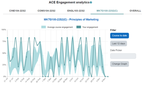
Figure 1: An example of ACE engagement analytics as displayed on the AKO|LEARN
ACE-3 Retention is a project aimed at adapting and applying a model commonly used in industry to analyse repeat purchasing behaviour which called the Pareto/NBD model. This model will be used to identify students at risk of dropping out by leveraging real student data, the University of Canterbury (UC) can implement this tool to create targeted strategies for improving student retention rates. Additionally, the ACE-3 program explores the model's effectiveness and potential applications in enhancing ACE’s analytics initiatives, ultimately supporting students throughout their academic journeys.
Higher Education (HE) is an essential component of society. Students enrolled in higher education institutions must be kept and graduate with a qualification that equips them for their desired vocation. Nonetheless, numerous students withdraw from university without obtaining their degree, resulting in increased financial burdens and diminished economic productivity for society (Muhammad et al., 2021). Student retention and achievement are key indicators of the success and validity of any university (Aljaloud et al., 2022; Aruna & Priya, 2021). Due to this fact, predicting such indicators with the help of machine learning has increased exponentially during the Covid-19 pandemic (Aruna & Priya, 2021). According to Organization for Economic Cooperation and Development (OECD), only 39% of students complete their degree programs within the expected time frame. Additionally, 12% of students registered for full-time studies are likely to drop out before they complete their second year of study, 24% by the end of the third year, and 20% by the time they finish their program (Okoye et al., 2024). The rate of student retention is generally defined as the number of students remaining enrolled in a university every semester or year in correlation with the graduation rates (Trivedi, 2022). Academic advising is expected to be crucial in facilitating academic integration and success for college students, particularly freshmen. Students at universities very often face the cumbersome and even emotionally exhausting task of choice of major, selection of the right courses, and preparation of an efficient class schedule (Buraimoh et al., 2021).
Understanding student's expectations and subsequent perceptions of the advising process, institutions may enact beneficial improvements in both service and quality, which may result in growing student satisfaction, retention, and higher graduation rates. By comprehending student's expectations and subsequent perceptions of the advising process, higher education institutions may implement advantageous enhancements in service and quality, leading to elevated student happiness, enhanced retention. The growing availability of student data and the heightened interest in forecasting student retention and success have prompted substantial efforts to employ traditional machine learning models for the efficient prediction of these metrics. University personnel would be better positioned to assist students in remaining enrolled and graduating on time by identifying those at risk of non-retention and determining the factors most influential in retention success. Timely support for students can assist academic advisors in helping those at risk of attrition remain in their original programs and achieve retention. This can help students in graduating on schedule with their desired degree and enable them to maintain their allocated scholarships. Precise data analysis and forecasts regarding student retention could assist academic advisers in identifying students who may be experiencing difficulties in their program and require assistance. However, as noted by (Attiya & Shams, 2023) accurately predicting retention rates across higher education institutions is challenging, as they are influenced not only by student interaction metrics but also by external factors.
This research aims to estimate the probability of student engagement within a course and examine its effect on student grades (fail/pass). It also emphasizes how important students continuously engagement within the course effect their achievement which will improve the retention of student in higher education and give an appropriate support for those at risk of failing/ dropping out the course. Therefore, this study was aimed to answer the following questions:
A large number of different models have been developed over decades to determine the likelihood of student retention using the realm of educational data mining and machine learning toward student performance (Jia & Mareboyana, 2013; Shafiq et al., 2022). The study by (Beech & Yelamarthi, 2024) examined the utilization of a deep learning model to forecast first-year student retention in engineering, achieving testing accuracies ranging from 66.7% to 95.2%. However, the imbalance of students with high grades complicates the model's ability to predict at-risk students, leading to a recommendation for oversampling. The research conducted by (Li et al., 2019) employs data science techniques on extensive educational data to elucidate the significant elements that inform models for predicting student retention. A robust correlation has been observed between student retention and both GPA and financial circumstances, which are recognized as significant predictors of retention outcomes. However, this study is inadequate in accurately capturing students who dropped out, with an accuracy rate of approximately 66%. The study by (Malatji et al., 2024) examines student retention among postgraduate students, focusing on the significance of factors that impede their application for postgraduate programs at the same institution where they completed their undergraduate studies. Utilizing various machine learning models, the Random Forest exhibited the highest accuracy at 95.62%. This model also identified similar factors contributing to students' non-retention in postgraduate programs, including years of registration, average marks, age, and possession of a sports scholarship.
The research of (Jia & Mareboyana, 2013) had used 11 features to predict retention over 6 years, including GPA, total credit hours, gender, age, distance from school and SAT score, with GPA bring the most influential in predicting retention. (Dreifuss-Serrano et al., 2024) examine the primary academic factors contributing to student attrition, including the academic workload during the initial semester, difficulties in adapting to a new learning system, vocational challenges, theoretical frameworks in the early semesters. It suggests colleges should emphasize both academic readiness and the holistic integration and emotional assistance of first-year students (McGhie, 2017). The study by (L. Kemper et al. 2020) attained an accuracy of 95.3% in forecasting student dropouts. Nevertheless, it just utilizes academic data, and the methodology fails to distinguish between pupils based on non-academic criteria. Similarly, (Segura et al., 2022) have shown dropout detection is not limited to enrolment variables, although it improves after the first semester, however, the study focused solely on first-year dropouts and included various degree programs but relied on the same limited set of features, which may hinder the accuracy of machine learning predictions. The study of (Dake & Buabeng - Andoh 2022) used a ML method to develop student dropout predictive model and to identify the features that are dominant impacting learners’ retention.
Various machine learning approaches, including Multilayer Perceptrons (MLP), Support Vector Machines (SVM), Random Forest (RF), and Decision Trees (DT), were employed to validate the model. (Delen, 2010) employed a multilayer perceptron artificial neural network (ANN) within a machine learning method to forecast student retention rates. Besides, (Uliyan et al., 2011) identified a risk of dropping out using a Deep Learning (DL) technique known as Conditional Random Field (CRF) along with a Bidirectional Long Short-Term Memory Model (BLSTM). The retention of students in higher education institutions is a significant issue that scholars are actively attempting to address globally.
One of the key problems in higher education is the lack of student engagement, which often leads to decreased academic performance, lower retention rates, and eventual dropout. Student disengagement can stem from several factors such as excessive study loads, insufficient academic support, or personal challenges. Timely support for students can assist academic advisors in helping those at risk of attrition remain in their original programs and achieve retention. This can help students in graduating on schedule with their desired degree and enable them to maintain their allocated resources.
In an increasingly digital world where much learning now takes place online, learning management systems (LMS) generate extensive metadata regarding students' academic activities, while demographic data is typically sourced from Student Management Systems (SMS) (Aljaloud et al., 2021). Since technology has reshaped learning styles, students are increasingly comfortable using digital tools in their studies. To support this trend, many higher education institutions have focused on LMS platforms, which enhance the learning experience by providing the key that opens the door to a wide range of resources and are believed to positively impact student engagement (Venugopal & Jain, 2015).
The variety of student engagement data available through the LMS can be used to identify patterns and trends in student engagement and performance. These can provide valuable insights into students who are at risk of dropping out and help educational institutions to perform interventions and support systems. The impact of the “Early Alert System” at the University of Canterbury, which uses nudging interventions when students are at risk of disengagement demonstrated that students who received a nudge reengaged at faster rate and spent more time engaging with online material (Kay & Bostock, 2023) .By addressing the needs of at-risk students, the university can enhance their efforts to improve overall student retention rates. By employing data analytics and predictive modelling, educational institutions can identify at-risk students in advance and provide them with the necessary support to help them re-engage in their studies. Additionally, understanding that “nudge” interventions can have wide-ranging effects across multiple courses opens the possibility of implementing these measures on a campus-wide scale.
Inspired by the “nudge” strategy in the University of Canterbury’s (ACE) system, this research introduces the Pareto/NBD model to provide a data-driven prediction method, enabling a quantitative analysis of student participation behaviour and offering theoretical support for targeted intervention strategies. The key motivation is the integration of customer behavioural prediction models within educational analytics, aiming to develop a more effective early warning and intervention tool for student learning behaviour.
The goal of this analysis is to evaluate the applicability of the Pareto/NBD model in the field of education and assess its effectiveness in predicting student learning behaviour and dropout probability. By employing this model, educational institutions can more accurately detect at-risk students, allocate resources optimally, and improve the efficiency and effectiveness of intervention measures, thereby enhancing student persistence and overall achievement.
The initial step of this analysis was to reproduce the results documented in "pareto_nbd_MATLAB" (Fader et al., 2005) using Python and subsequently apply the same approach to the real UC student data. There are two sample datasets were used to implement the Pareto/NBD model (Fader et al., 2005) by converting MATLAB code into Python code. Table 1 and Table 2 provide a brief description of each variable in the two datasets. The "cdnow_dataset" was primarily used for parameters estimation, while the "cdnow cumulative dataset" was used to measure the estimation and prediction performance. These sample data lay the foundation for the subsequent analysis.
| Variable | Description | Type |
|---|---|---|
| ID | Unique identifier for each customer. | Integer |
| FREQ | Frequency of transactions made by the customer during the observation period. This represents the number of repeat purchases. | Integer |
| RECENCY | The time of the most recent transaction relative to the start of the observation period. | Numeric |
| T | Total time the customer was observed during the study period. | Numeric |
| p2x | Represents the number of transactions made by each customer in the following 39-week period after the observation period (up to week 78). | Integer |
| Variable | Description | Type |
|---|---|---|
| Time | Represents the time period (e.g., weeks) since the start of observation. | Numeric |
| Count | Cumulative number of transactions or events recorded by the end of each corresponding time period. | Numeric |
The data included in this study was sourced from two databases of University of Canterbury (UC) students. The initial source is student data (Jade_source), which contains records from the student system documenting enrolment and withdrawal from courses. Furthermore, this documented student performance metrics like GPA, grades, and demographic information (gender, age, etc.). The second source originates from the UC Learning Management System (LMS), which serves as the "blackboard" for students to engage with their courses online which is USER and AKO|LEARN dataset. To map these tables and associate students with their results and interactions, the student_id field was used, which was hashed to protect privacy. Additionally, to prevent mismatches between the student data and the Learn system data, the analysis was restricted to a specific course by filtering both tables using course_code and course_id, ensuring proper alignment during the joining and processing stages (Figure 2).
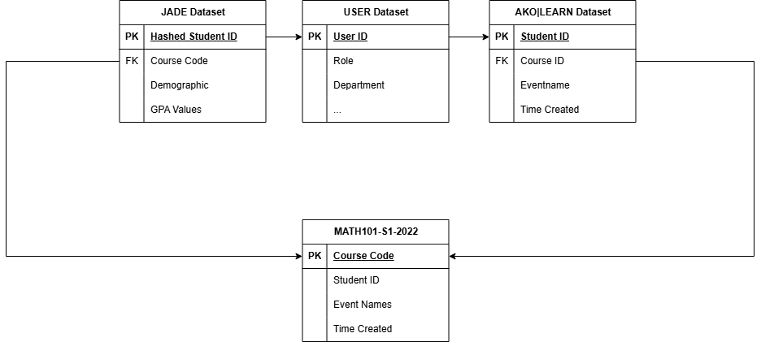
Figure 2. Entity-Relationship Diagram of Data Sources and Integration Process
Initially, our objective is to forecast outcomes for all courses recorded in the LMS system; however, because to time constraints, we will focus on a single course as a baseline measurement, from which future research can be extrapolated to other courses. The original dataset comprised the courses MATH101-22S2 and STAT101-22S2 due to their discernible patterns and well-organized structures. Nonetheless, there were significant missing GPA data, complicating the feature engineering process, especially as GPA is likely a crucial feature. Despite imputation, the substantial volume of missing data may adversely affect model performance, possibly due to data entry complications. Furthermore, many classes, like STAT101-22S2, comprise approximately 949 individuals, yielding a comparatively extensive dataset. Analysing this data can be both time-consuming and computationally demanding. Consequently, we chose MATH101 – 22S1 for our study as it encompassed all the requisite aspects for our research.
Jade student data indicates that 572 students are enrolled in this course, matching to 570 unique IDs, suggesting that two students possess dual enrolment statuses. The first student's course enrolment status was WDFR (Withdraw with Full Refund) for both on-campus and remote enrolments. The second student's status was WDFR for the campus option, while it indicated enrolment for the distance option. In this instance, we preserved solely the distance-enrolled record for the second student, resulting in a dataset including 569 unique student IDs. Upon merging with the Users database from LMS (log_data), the student count was reduced to 566, indicating a discrepancy between the two tables and that three students have not been assigned in the LMS system. Consequently, while our model utilized student interactions within the LMS, we exclusively consider those students whose IDs are documented on Learn. Subsequently, we merge our dataset with the log store table on LMS data, which documents all student interactions, and quantify the frequency of their engagement in this particular course. In this scenario, we assume that each interaction by students on the LMS system is logged as a single occurrence. Consequently, 23 students are listed in the LMS system but exhibit no recorded attendance. We presume that upon enrolment in the course, each student should immediately register one instance of attendance on the inaugural date of the course.
This assists the model in effectively identifying patterns of students who may not succeed in the course. The data was truncated to align with Semester 1; according to UC's Academic Report 2022, Semester 1 spans from February 17, 2022, to June 25, 2022. Table 3 provides features and the description from the final data frame before applying filters and conducting model training.
| Source Data | Column Name | Description |
|---|---|---|
| JADE_PROJ_UNSNAPPED join MDL_PROJ_USER |
USER_ID | Unique identifier for each user or student in the dataset. |
| GPAVALUE | Grade Point Average (GPA) value representing the user's academic performance. | |
| JADE_PROJ_UNSNAPPEDFTS | GRADE | Grade achieved by the user (e.g., "A," "B," etc.). |
| GRADERESULT | Outcome of the user's grade evaluation (e.g., "Pass," "Fail"). | |
| MDL_PROJ_LOGSTORE | EVENTNAME | Name of the event or activity performed by the user (e.g., "course_viewed"). |
| TIME_CREATED | Time when the event or activity was logged in the system. | |
| DAILY_FREQUENCY | Number of times the user engaged in the specific activity on a given day. |
Building upon the dataset described in the previous section, Exploratory Data Analysis (EDA) was conducted to gain insights into the characteristics and quality of the data, as well as to identify patterns and relationships relevant to the study's objectives.
The first step in the EDA involved performing descriptive statistics, it provided a summary of data distribution. Table 4 below calculate the descriptive statistics which tracks the number of interactions recorded per day by students on LMS system.
| TOTAL_CLICKS_PER_DAY | |
|---|---|
| count | 27050 |
| mean | 52.644 |
| std | 70.45 |
| Min | 1 |
| Max | 1357 |
| 25% | 4 |
| 50% | 20 |
| 75% | 80 |
According to table 4, while some students are highly active, others shown the minimal engagement. The wide range and high standard deviation suggest that further investigation into student behaviour such as grouping demographic factors or GPA may be valuable for understanding patterns.
Figure 3.1 indicates a distinct rise in contact within the initial two weeks following the commencement of the course. The significant increase, especially during the second week, peaking at over 180,000 total clicks, can be ascribed to the preliminary engagement period in which students investigate course contents, acclimate to the platform, and determine their continued enrolment in the course. This timeframe is pivotal, coinciding with the decision-making period during which students either enrol in or withdraw from the course, as indicated by the previously outlined enrolment trends. After the first engagement peak, interactions stabilize but experience a modest fall in the following weeks, maintaining consistent activity throughout the middle of the term. A secondary surge arises during Week 8, presumably linked to mid-term examinations and quizzes. During this time, students typically enhance their interaction with the LMS to get resources, prepare for evaluations, and complete assignments. Between Week 9 and Week 11, there is a marked and substantial decline in interactions. This interval coincides with the term break, during which student engagement on the LMS markedly diminishes. The term break permits students to suspend their academic obligations, which is evidenced by the data indicating low involvement levels. Near the end of the course, there is a further surge in LMS activity, signifying the preparation phase for the final examination. During this period, students diligently engage with course materials, prepare for examinations, and finalize any outstanding assignments or projects. This phase is characterized by a modest yet discernible rise in involvement relative to the mid-term apex, as students concentrate their efforts on successfully completing the course.
Similarly, Figure 3.2 shown the number of students interact each week during the course. Based on the plot, students start to engage fast just right after the first week of the semester, these also consider as a top period where students engage most during the course, simply because they want to explore the course content and decide to stay or leave the course at the beginning. The frequency keep stabilize after weeks with the significant drop during the term break. Students begin the second term actively but not as frequently as the first term, this might indicate several students drop out from course silently after the break.
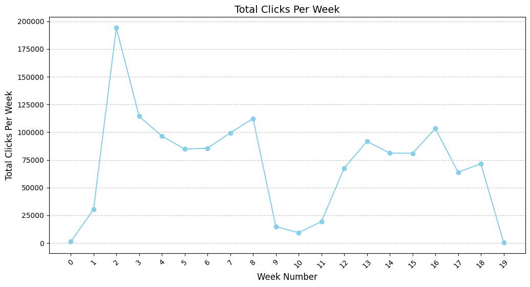
Figure 3.1 Students total clicks per week
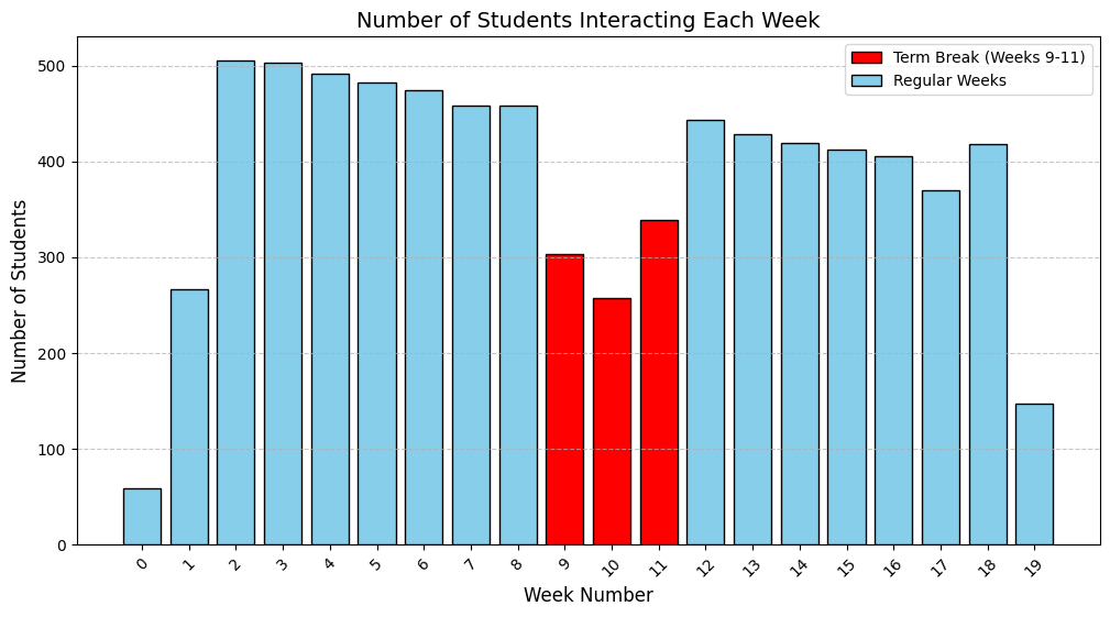
Figure 3.2 Students interactions per week
Based on Figure 4.1, the total frequency of interactions on the LMS shows a wide variation across different GPA values. Students with low interaction frequencies tend to have lower GPA values. For instance, students with a GPA between 0 and 2 are primarily clustered within the 0 to 2000 frequency range. This indicates a potential correlation between low engagement and lower academic performance. As the GPA increases, the interaction frequency tends to be higher. For example, students with a GPA in the range of 6 to 8 are more commonly observed with interaction frequencies between 3000 and 6000. This pattern suggests that students who are more engaged with the LMS are likely to perform better academically. This observation is further supported by Figure 4.2, which shown the correlation between student GPA and their frequency. The high correlation score (0.69) indicates there is a strong positive relationship between GPA and there frequency, in another words, student’s with high interaction on LMS tend to have higher GPA value. This reinforces the importance of consistent engagement with the LMS as a factor influencing academic success.
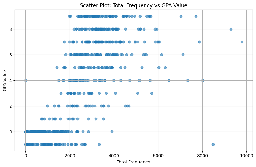
Figure 4.1 Relationship Students Frequency & GPA
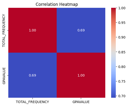
Figure 4.2 Correlation Heatmap
Figure 5 illustrates a significant relationship between students’ grades and their average total frequency of clicks, indicating that higher average total frequency corresponds to higher grades. Students earning top grades (e.g., A+ and A) typically exhibit more clicks. By contrast, students with lower grades (e.g., C-, D, and WD) tend to have fewer clicks. Specifically, students who receive a WD (Withdraw) record the lowest average number of clicks, likely because they stop interacting with LMS at an early stage or drop out altogether, becoming “inactive” users. As we can see in Figure 5, students have “A” grade tend to have the same interaction level with not large variate compared to other where the huge fluctuation in frequency effect the grades. Moreover, there are several outliers in each range of grades, this highlights several students although interact on LMS frequently but obtained a lower grade and otherwise.
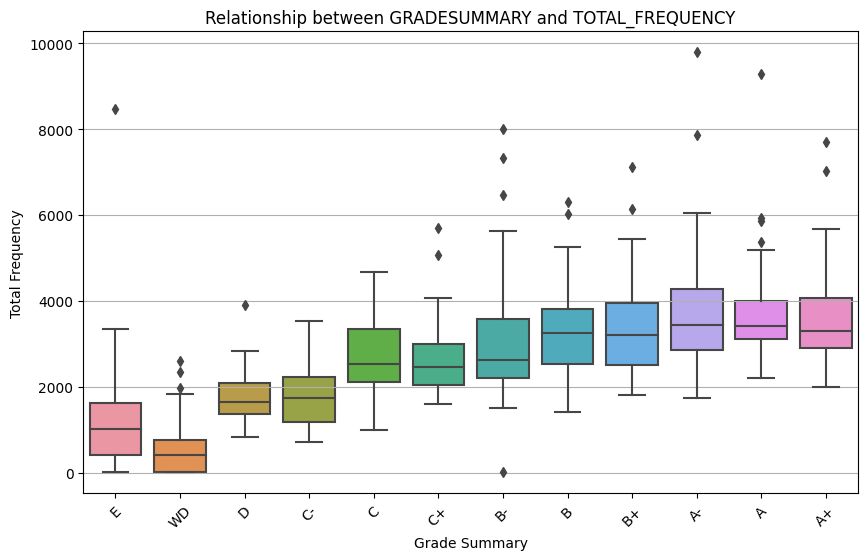
Figure 5. Average total frequency by grade
The proportion between student grade results and their age groups as shown in Figure 6 indicates a distinct trend between the age spectrums. Students under the age of 20 have the largest group in the dataset with a significant portion of falling their course. This highlighted the potential need for targeted interventions for younger students since this is their first year in higher education with several confusions. On the other hand, although the number of failing students slightly exceeds those passing, students which in 20 – 24 age group shown a relatively balanced distribution between pass and fail outcomes. At older groups such as 25-29 and 30-54 years, the number of students is getting smaller but the pass/ fail ratio more balanced. Curiously, there is a complete absence of failures among students 55 and older, despite the fact that the sample size is extremely small for this age group. As a result, this plot shown age also is a potential factor effect the academic outcome and suggest that younger students consider as an at – risk group where need an academic support.
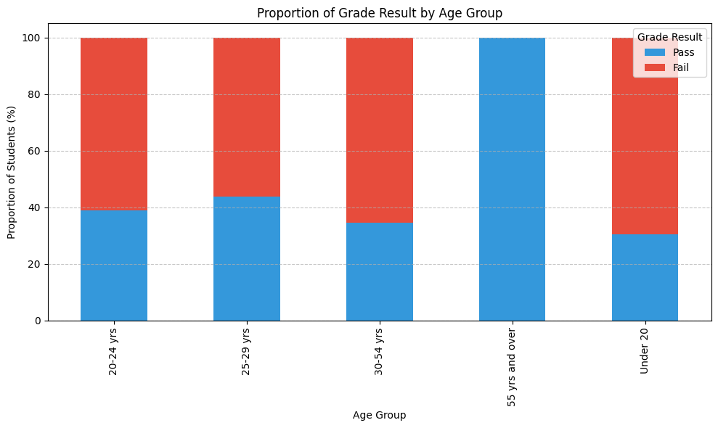
Figure 6. Proportion Between Student Grade and Age Group
These findings provide a basis for further analysis by identifying characteristics that are most correlated with academic outcomes and suggest areas for further investigation. The differences identified in engagement and performance highlight the need for targeted interventions, particularly for at-risk populations such as younger students or those exhibiting reduced LMS engagement. By estimating the probability of student survival based on these characteristics, this study uses student outcomes as a benchmark to understand the impact of survival probabilities on academic achievement. Given that GPA is a critical measure of student success, it will serve as the primary indicator to categorize student outcomes into groups for simplified analysis and prediction. The categorization is outlined below:
| GPA Value | Grade Summary |
|---|---|
| 9, 8, 7, 6, 5, 4, 3, 2, 1 | Pass |
| 0 - 1 | Fail |
Customer Lifetime Value (CLV) Analysis comes from an industrial business model that predicts the net profit attributed to the entire future relationship with a customer. It enables businesses to identify customers who are more likely to make purchases and develop strategies to retain them (Megantara et al., 2023). CLV operates in two types of customer interaction contexts which is contractual and noncontractual. A “contractual” setting is one in which customers are explicitly obligated to engage with the business for a certain period, such as paying for a subscription service like Netflix. In contrast, a “noncontractual” setting refers to a business customer interaction context in which there is no formal contract compelling customers to continue making purchases. This emphasize the noncontractual settings where there is no binding agreement, make retention prediction more challenging. In the context of education, predicting student retention can be seen as analogous to customer retention in noncontractual settings, as students are not formally obligated to remain engaged throughout their academic journey.
In order to analyse the customer lifetime value (CLV), the RFM analysis which segments customers based on Recency (R), Frequency (F), and Monetary Value (M) had been used as essential features for estimating probabilities of customer will make the purchase in the future. These features summarize customer behaviour patterns as follow:
Over the years, several adaptations of the RFM model have been developed for different purposes. For instance, the RFD model (Recency, Frequency, Duration) was designed to examine consumer behaviour related to activities like viewership, readership, or product browsing. In 2009, Yeh et al. introduced the RFMTC model (Recency, Frequency, Monetary Value, Time, Churn Rate) which was based on RFM model. Another version called RFM-I (Recency, Frequency, Monetary Value – Interactions) that integrates marketing interactions by considering the recency and frequency of client engagement (Tkachenko, 2015).
In this study, we will apply the RFD analysis where Duration (D) replaces Monetary Value to better represent student engagement patterns to analyse student behaviour in the ACE project, using data from the University of Canterbury. In this context:
| Frequency (x) | An observed count of interactions (e.g., clicks on the LMS) made by a student during the observation period |
| Recency (t_x): | Duration from the course start date to the last active date within observation period. |
| Duration (D) | An observation period |
| Transaction rate (λ) | Total frequency of student clicks on the LMS (e.g., daily event counts). |
| Dropout rate (μ) | Likelihood of a student withdrawing, failing to engage, or leaving the institution |
The RFD model, by the integration of these factors, facilitates a more sophisticated comprehension of student behaviour, hence allowing for the predicting of engagement and retention trends. This analysis establishes the basis for employing the model, discussed in the following section, to estimate the likelihood of a student remaining engagement ("alive") in the course.
Pareto/NBD (Negative Binomial Distribution Model) produced by (Schmittlein et al. 1987) is a probabilistic model built for noncontractual settings method that originated from Customer Lifetime Value (CLV) analysis, it uses to estimate the probability of customer being active at the end of an observation period and there expected number of purchase in the future. In this study, we will implement the Pareto/NBD model to estimate the probability of student being engaged (alive) within the course drawing inspiration from its original application in customer retention.
Based on the model, each student’s activity (e.g., students interact on LMS) is assumed to follow a Poisson process, where the activity rate (λ) is unique to each individual. The likelihood of a student dropping out from the course will follows an exponential distribution with dropout rate μ (Schmittlein et al. 1987). In order to account for the variations in individual behaviour, both activity rate (λ) and dropout rate (μ) are assumed to follow the Gamma distributions (Heterogeneity):
The r, α, s, β are critical since they define the Gamma distributions that account for heterogeneity across students. The table below describe those parameters and it usability.
| Parameter | Usability | Description |
|---|---|---|
| r | Determines the variability in how frequently students interact with the LMS. A higher r value implies less variability in transaction rates across the student population | This parameter is a shape parameter of the Gamma distribution for the transaction rate (λ) |
| α | Controls the average transaction rate. It reflects the overall tendency of students to engage actively with the LMS | This parameter is a rate parameter of the Gamma distribution for the transaction rate (λ). |
| s | Determines the variability in dropout rates across students. A higher “s” value implies less variability in how likely students are to disengage | This parameter is a shape parameter of the Gamma distribution for the dropout rate (μ). |
| β | Controls the average dropout rate. It reflects the overall tendency of students to disengage or withdraw from the course | This parameter is a rate parameter of the Gamma distribution for the dropout rate (μ). |
In this project, the likelihood estimation process was then used to find the set of parameters (r, α, s, β) that maximize the likelihood function which is designed to estimate the likelihood of a student remaining engaged (“alive”) in the course based on their observation interact with LMS. The likelihood function integrates over the Gamma distribution transaction and dropout rates where it is combining the probabilities of observed frequency (x) and recency (tx) of interactions as well as the probability of student remaining engaged by the end of the observation period (T). The total log – likelihood was then sum of the individual log – likelihoods across all students in the dataset. As a results, it ensures the parameters (r, α, s, β) are optimized where it satisfies the maximum the agreement between the model predictions and observed data. By following the paper from (Schmittlein et al. 1987), key formulas include:
After defining Gamma distributions for λ and μ, the next step is to integrate these distributions into the full likelihood function. The process involves combining the transactional likelihood, the survival probability and the Gamma prior for λ and μ.
$$ P(x, t_x, T \mid r, \alpha, s, \beta) = \int_0^\infty \int_0^\infty P(x, t_x \mid \lambda) \times P(\text{Alive at } T \mid \mu) \times g(\lambda \mid r, \alpha) \times g(\mu \mid s, \beta) \, d\lambda \, d\mu \tag{5} $$
The log – likelihood function is maximized to efficiently explore the parameter space and determine the values of r, α, s, β that best fit the data. These parameters are crucial for estimating the probability of a student remaining engaged, guiding predictions and interventions for student retention.
After formulating the Pareto/NBD model, it is crucial to estimate the parameters r, α, s, and β that optimize the likelihood function. This research utilizes two methodologies to do this: the Nelder-Mead technique and Nested Bayesian Sampling. Each method presents distinct advantages and obstacles, which are elaborated upon below.
The Nelder-Mead simplex algorithm is a widely used direct search method for solving unconstrained optimization problems. The algorithm starts with an initial simplex comprising points in the search space. At each iteration, the algorithm evaluates the objective function at the simplex vertices and applies geometric transformations like reflection, expansion, contraction, or shrinkage to improve the function values. Known for its simplicity and effectiveness in lower dimensions, the method struggles with efficiency and convergence in high-dimensional problems. Modifications such as adaptive parameter tuning have been introduced to enhance its performance in these scenarios (Gao & Han, 2012).
In this study, the Nelder-Mead method performed well on the sample data, closely approximating the target results. However, it failed to find the optimal parameters for the real data, likely due to the high dimensionality and poor initialization of the student data. This method could have achieved better results if more time were available
The primary estimation method in this study was Nested Bayesian Sampling, which was implemented to mitigate the constraints of Nelder-Mead and more accurately quantify parameter uncertainty. Bayesian inference employs probability to quantify the degree of uncertainty in predicting model parameters. When it comes to parameters, Bayesian approaches view them as random variables governed by probability distributions, as opposed to the fixed values used by statistical methods (Hooten and Hefley, 2019; Muth et al., 2018). Bayesian models possess two fundamental qualities. Probability distributions are utilized to express unknown quantiles, referred to as parameters. Bayes' theorem is utilized to revise parameter values according to the existing data.
By using probability distributions to incorporate prior knowledge, Bayesian inference offers substantial advantages. According to (Lemoine, 2019 & Banner et al., 2020), these prior distributions can either represent mathematical formulas that are instructive based on previous research, or they can suggest feasible parameter ranges when there is limited prior information. The posterior outputs generated by this method explicitly account for the uncertainty and variability in projected outcomes (Neal, 2004) by providing quantitative distributions and ranges for parameter estimations. Bayesian inference treats parameters as random variables governed by probability distributions. Unlike traditional optimization methods that yield single-point estimates, Bayesian approaches provide posterior distributions that reflect both prior knowledge and observed data. Bayes’ theorem updates the prior distribution with the likelihood to obtain the posterior distribution.
$$ P(\theta \mid \text{data}) = \frac{P(\text{data} \mid \theta) P(\theta)}{P(\text{data})} \quad ; \quad \text{where } \theta = (r, \alpha, s, \beta) \tag{6} $$
Building on the principles of Bayesian inference, Nested Sampling provides an efficient computational method for estimating Bayesian evidence (Z) and posterior distributions. Originally proposed by (Skilling, 2004), Nested Sampling integrates the prior by dividing it into nested of constant likelihood. Instead of only providing samples proportional to the posterior, as Markov Chain Monte Carlo (MCMC) methods do, Nested Sampling estimates the evidence and the posterior simultaneously. It also has many attractive statistical properties such as stopping criteria for termination of sampling, producing a series of independent samples, flexibility to sample from intricate, multi-modal distributions, capability to determine the influence of statistical and sampling errors on findings from a singular execution, and simplicity in parallelization (Dynesty 2.1.5 Documentation, n.d).
In this study, Nested Sampling was employed to analyse student interaction data from the LMS system, collected at various points throughout their academic courses using the Dynesty package with implement in Python. This approach had also been used in prior studies (see Corbett and Anderson, 1994; Mao et al., 2018; Cui et al., 2019) to demonstrate the value of educational data at different intervals, such as through evaluations and interventions.
Figure 7 shown the method workflow in order to accomplish the objective of this study.
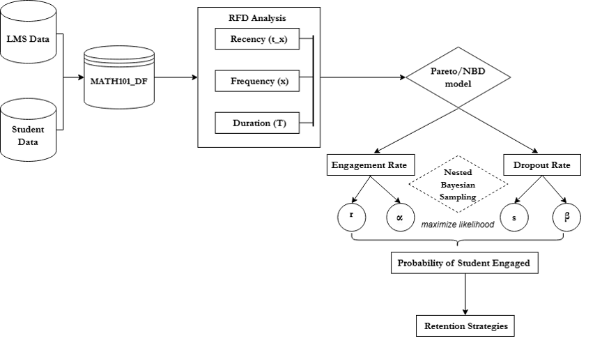
Figure 7. Workflow for Modelling Student Engagement and Dropout Rates Using the Pareto/NBD Frameworks
The probability of engagement for each student was calculated to identify individuals with a low likelihood of remaining engaged in the course. This information was used to design timely intervention strategies, such as sending targeted messages to re-engage students, with the goal of improving their performance and course completion rates. The probability of engagement wad derived based on (Fader et al., 2005) which mathematically expressed as follows:
$$ P_{alive} = \frac{\mathcal{L}(\text{engaged})}{\mathcal{L}(\text{total})} \tag{7} $$
Explanation of Components:
Represents the likelihood of a student remaining engaged in the course. This value is determined based on four key parameters (r, s, α, β) and is calculated using:
$$ \mathcal{L}(\text{engaged}) = \frac{s}{r+s+f} \times {}_2F_1 \left( r+s+f,\ s+1,\ r+s+f+1,\ \frac{|\alpha - \beta|}{\alpha + R} \right) \tag{8} $$
This method adapts principles from customer lifetime value (CLV) modelling to a student engagement context, allowing for a robust prediction of engagement based on interaction data. By using parameters such as frequency and recency of student interactions, the model provides a probabilistic measure of engagement. Therefore, students with low probability were flagged for intervention and allow educators to retain them with tailored strategies.
To determine the optimal period that student might dropout, we perform the grid search to look at different combination of observations period (T) and the frequency threshold (X). In this scenario, the observation period (T) was defined from after the course start one week since this is the stable time where students finish there add/ drop period to the end of the course. Since students have different number of interactions within the course, the frequency threshold (X) is a user’s daily frequency that use to determine whether the users are considered as active on a given day within the observation period (see Figure 8). This threshold helps identify each user's last activity date, which represents the most recent day within the observation period when their activity frequency exceeded the threshold. The Recency is calculated as the difference between the user's first interaction day and their most recent day of activity. To determine the optimal activity frequency threshold (X) for classifying users as active in this course, a range is chosen between the 20th percentile (X=3) and the 80th percentile (X=99) with the step size of 5 between combinations. This range ensures a focus on identifying an activity frequency that yields the best results for the analysis.
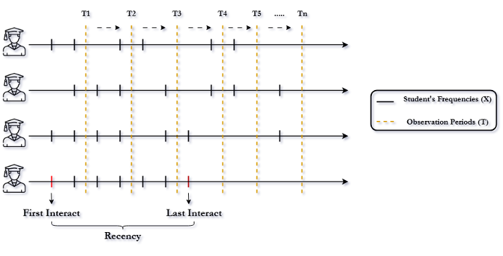
Figure 8. The Example of Student Interaction Frequency Timeline and Observation Periods
Based on Figure 8, the observation period (T) had been shifted after weeks to find the optimal combination of Frequency and Recency. For training purposes, the daily frequencies are summed into a total frequency for each user. There are some special cases in which certain users do not have any day in the observation period on which their frequency exceeds threshold. For these users, their last active date is set to the day with the highest frequency recorded during the observation period (case 2, Figure 9). If multiple dates have the same highest frequency, the date closest to the end of the observation period is selected as their last active date (case 1, Figure 9).
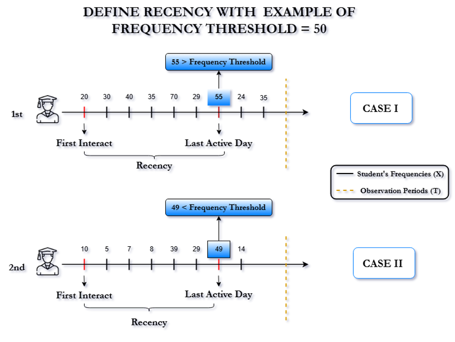
Figure 9. Defining Recency with Examples of Frequency Thresholds
From the Pareto/NBD model, the probability of being “alive” represents the likelihood that a customer (or in our case, a student) will continue to engage in the future. When applying this model to student data, finding the optimal parameters to maximize log-likelihood is crucial for estimating the probability that each student remains “alive” after the observation period (T). This probability informs whether the student may “withdraw” or “fail” from the course. In our study, the student’s grade result (Pass/ Fail) will be used to explore this relationship.
However, the optimal combination of the frequency threshold (X) and the observation time (T) was guided by the goal of maximizing the Recall metric. The Pareto model was initially used to compute the probability of students being engaged (alive) based on their frequency of interactions, recency, and observation time. This probability provides an estimate of the likelihood of students remaining engaged in the course. Instead of relying on the log-likelihood, which is the default metric in the Pareto model, the Recall was prioritized as the primary evaluation criterion. The rationale for this decision is rooted in the study's objective that identify as many students as possible who are at risk of disengaging from the course and potentially failing, therefore, timely interventions or nudges can be deployed to retain them. Moreover, as the observation period increases, the additional data may contain noise or irrelevant patterns that do not contribute meaningfully to the goal of identifying at-risk students. This noise can inflate the log-likelihood score, making it less reliable to predicting disengaged students.
Through a systematic exploration of the observation period which shifting the weekly intervals to identify optimal timings for interventions, the study uncovered that both week 6 and week 7 with the frequency threshold yield that highest recall, however, the AUROC on week 7 is higher than week 6 which indicates that week 7 provides a better balance between sensitivity and specificity, meaning it can more effectively distinguish between positive and negative cases. According to week 7, the model obtained a Recall of 0.89 and an AUROC of 0.74. These metrics demonstrate the model’s strong capacity to detect students at high risk of failing where it is capturing nearly 89% of such case with minimal false negatives (Figure 10).
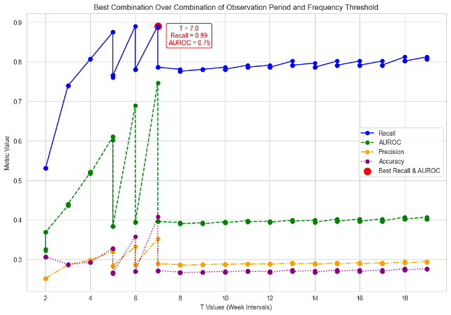
Figure 10. Metrics Comparison Across Observation Periods to Identify Optimal Intervention Timing
The Recall score highlights the model’s effectiveness in identifying vulnerable students, this help reducing the likelihood of missing individuals needing for timely interventions. Concurrently, the AUROC of 0.74 reflects a well-maintained balance between sensitivity and specificity, allowing the model to distinguish between students likely to succeed and those at risk accurately. As a result, this combination underline at week 7 as an optimal period for proactive retention strategies since the model can identify as many students fail from the course as possible.
Following the determination of week 7 as the optimal period for at – risk identification, the probability of student engagement was examined to provide a deeper insight into individual students’ likelihood of engaging in the course. The study used parameters (r, s, α, β) of the combination between the optimal observation period and the frequency threshold to calculate the probability of engagement for each student (see formula 7 & 8). These probabilities were visualized through the posterior distributions where the probability was then identified by maximum a posterior (MAP) as illustrated in figure 11.
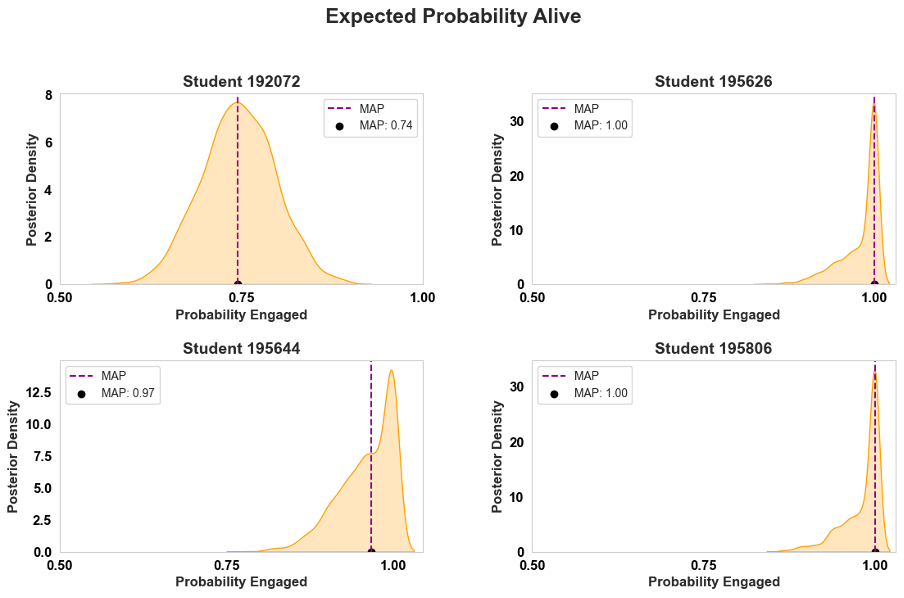
Figure 11. Posterior Distributions of Probability of Engagement for Selected Students
These visualizations depict the posterior densities of the probability engagement for four example students, this enabling an in – depth understanding of individual engagement likelihoods. For instance, students 192072 displayed a MAP estimate of 0.74, indicating a moderate probability of being engaged. On the other hand, students 195806 and 195626 achieved MAP estimates of 1.00, signifying a very high likelihood of continued engagement. The variation across students shown the model’s precision in differentiating levels of engagement. Besides, the probabilistic insight offered by these play a significant role in empower educators to prioritize targeted interventions for students with lower engagement probabilities, where higher education can enhance overall course outcomes and mitigating dropout rates as well as improve student achievement.
To understand the contribution of various features which including the probability of engagement derived from the Pareto/NBD model, a Random Forest classifier was employed to predict students final grade outcomes (Pass/Fail). Unlike other linear models, Random Forest can capture nonlinear interactions between predictors and account for high order effects, besides, Random Forest also provides interpretable insights into feature importance by averaging the reduction in impurity (e.g Gini index, Entropy) across all trees making it ideal for identifying the most impactful predictors without considering the correlation between features.
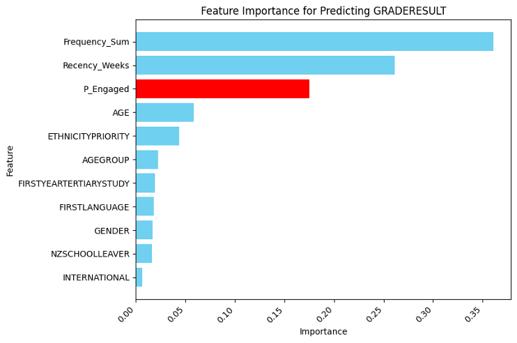
Figure 12. Random Forest Feature Importance for Predicting Student Grade Outcomes
The analysis revealed that Probability of Engagement ranked among the top three most important predictors of student’s grade outcome (Figure 12). The top three features were: the frequency of interactions, representing the total number of engagements students had within the course; the recency, reflecting how recently students interacted with the course; and the Probability of Engagement, which captures the likelihood of a student remaining actively engaged, as derived from the Pareto/NBD model. This finding highlights the importance of continuous engagement in predicting student success. Notably, Probability of Engagement emerged as a critical factor, outperforming other demographic variables such as Age, Ethnicity, and Gender, reinforcing the importance of engagement-related metrics over static demographic features.
The inclusion of probability of engagement as a feature provided significant predictive power, demonstrating its relevance in understanding student outcomes. Its high importance, second only to Frequency and Recency. This finding highlights the necessity of fostering continuous engagement throughout the course duration. Students who maintain consistent interactions patterns are more likely to succeed academically. By integrating probability of engagement into predictive models, higher education institutions can distinguish whose engagement probabilities are declining and intervene before disengagement leads to failure. For example, targeted interventions such as personalized reminders or motivational messages could be deployed to re - engage at risk students. Moreover, the impact of engagement metric over the student demographic features indicates the need for course design that emphasize active participation rather than relying solely on demographic predictors. Therefore, this highlight the need to create the learning environment where success is driven by student behaviour and engagement rather than there pre – existing characteristics.
Parameter estimation was the most time-consuming phase of the analysis. Multiple factors influenced the optimal parameter values, such as the initial guess, parameter bounds, choice of optimization methods, length of the observation period, and the threshold used to classify a user as active. Given that the training dataset contains its typical features, it is worthy to experimenting with different methods. Since the training dataset exhibits typical characteristics, experimenting with different optimization techniques remains a valuable approach.
Through this study, we successfully identified optimal parameter values using the nested sampling method. However, when applying other optimization methods, such as L-BFGS-B (Limited-memory BFGS with Bounds) and Powell’s method, we were unable to find optimal results due to time constraints. This suggests that further refinements and alternative approaches could enhance parameter estimation.
For future work, two key directions can be explored. First, additional parameter tuning should be performed on the existing methods to refine results. Second, alternative parameter estimation techniques should be investigated to identify the most suitable approach for this dataset. Potential methods include Markov Chain Monte Carlo (MCMC) and Genetic Algorithms (GA), both of which could provide more robust optimization outcomes.
Given more time, there is significant potential to further refine parameter selection and optimization strategies. Exploring advanced estimation methods and improving computational efficiency could lead to more accurate and reliable parameter values, ultimately enhancing model performance.
One key limitation in this study is that different courses exhibit varying student learning patterns, making it difficult to implement a single model that performs well across all student data. This necessitates the exploration of different optimization techniques and hyperparameter tuning to identify the best-performing model for each dataset. While the Pareto/NBD model remains a promising approach, it may be more suitable for certain courses than others, depending on the learning behaviors observed in those courses.
Additionally, this study focuses specifically on first-year university courses, and there are approximately 751 different 100-level courses at the University of Canterbury. The quality and completeness of data from these courses vary, which can significantly impact model performance. In particular, missing or inconsistent data could reduce the model’s effectiveness.
A valuable direction for future work is to extend this approach to additional datasets across various courses and academic levels. To enhance model robustness and accuracy, future studies should place a strong emphasis on data preprocessing, including rigorous data cleaning and theoretically grounded imputation methods for handling missing values. By improving data quality and optimizing model selection for different learning patterns, the university could extend the applicability of this approach to a broader range of students, ultimately maximizing its impact on student success.
The Pareto/NBD model is widely used for customer-base analysis, but its applicability depends on the assumption of heterogeneity within the dataset. If this assumption does not hold, the model may not fit the data well, potentially affecting predictive accuracy.
To address this limitation, alternative models such as BG/NBD (Beta-Geometric/Negative Binomial Distribution) could be explored. Unlike Pareto/NBD, BG/NBD accommodates discrete-time behavior, which may be more suitable for certain datasets. Additionally, other hierarchical models could be investigated, such as incorporating GPA as a covariate to influence key parameters like λ (purchase rate) and μ (dropout probability).
Future work includes, first, exploring the applicability of other alternative models to determine whether discrete-time behavior better captures student engagement and retention patterns. Second, exploring hierarchical models by incorporating additional features to assess their impact on dropout probabilities. Third, applying these new models to different student datasets to evaluate which model performs best under various conditions.
This study had successfully applied the business model Pareto/NBD into the educational context to estimate student engagement probabilities and predict at – risk students in a university course. Additionally, by using data from University of Canterbury (UC) Learn Management System and Nested Sampling as an optimization method, the model effectively identified optimal intervention period, particularly week 7 where is the effective time to detect student at risk during the course. Besides, this study also emphasizes student continuous engagement on the Learning Management System (LMS) is a key determinant of student success with the probability of engagement ranking among top 3 predictive factors for academic outcomes. As a result, it highlights the need for early intervention strategies such as personalized nudges to re – engage students at risk of failing as well as the importance of course design based on student interaction as a key factor of succeed alongside other characteristics. By integrate this study into practical, higher education can proactively improve student outcomes and enhancing retention rates.
The authors would like to thank the University of Canterbury for providing the data and resources necessary for this research. We also acknowledge the contributions of our colleagues in the ACE project for their valuable insights and support throughout this study.
We would like to express my sincere gratitude to my supervisors, Paul Bostock and Nicki Cartlidge for their guidance and support throughout this project. Their expertise and feedback have been instrumental in shaping the direction and quality of work.
THANK YOU FOR READING!