BACKGROUND
This project builds a complete end-to-end MLOps workflow using real-world Chicago Taxi Trips data. It covers everything from data ingestion and exploratory data analysis to experiment tracking, model deployment, and monitoring using modern tools like MLflow, Mage, AWS S3, Docker, and Evidently.
I. INTRODUCTION
The Chicago Taxi Trips dataset is a rich source of information about taxi rides in Chicago, including pickup and drop-off locations, timestamps, trip distances, and fare amounts. This project aims to build a machine learning model to predict taxi fares based on these features, providing valuable insights for both taxi operators and passengers.
II. DATASET
The dataset consists of over 1.5 million records of taxi trips in Chicago, collected from the City of Chicago's open data portal. Each record includes features such as pickup and drop-off locations, timestamps, trip distances, and fare amounts. In order to ingest the data , I have used the python script to ingest the data via request library and store it in the local directory.
III. MLOPS PIPELINE
1. Data Ingestion & Exploration
The first stage of this project focused on acquiring and understanding the Chicago Taxi Trips dataset, a large and diverse collection of trip records from the city’s open data portal. To ensure reliability and reproducibility, I implemented an automated process to fetch and store monthly data in an efficient Parquet format, providing a consistent foundation for downstream analysis.
Once the data was ingested, I carried out an exploratory analysis to assess quality, engineer meaningful features, and uncover patterns that could influence trip duration. This involved creating variables such as trip distance, time of day, day of week, and weekend indicators, alongside parsing timestamps for temporal insights.
A preliminary RandomForest model was used to gauge feature importance, revealing key drivers like distance and location attributes. Visual analysis highlighted trends in trip durations across weekdays, differences between trips with complete and missing location data, and the relative influence of various predictors. By the end of this phase, the dataset was clean, enriched, and well-understood, providing a strong analytical foundation for model development in the subsequent stages of the MLOps pipeline.
1.1 Trip Duration Distribution
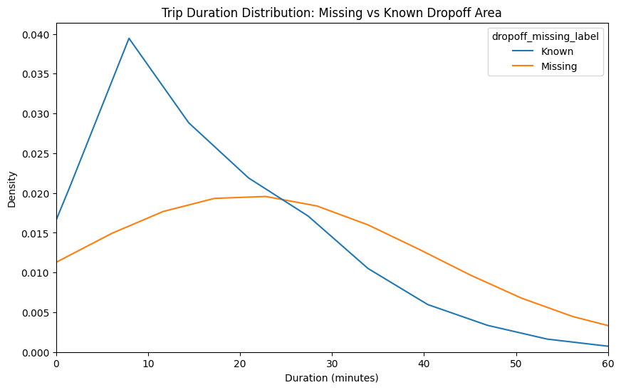
One of the key findings from the exploratory analysis was the relationship between missing drop-off location data and trip duration. By comparing the distributions of trips with known versus missing drop-off areas, it became clear that records with missing information were more likely to represent either very short or unusually long trips. In contrast, trips with known drop-off areas tended to cluster around typical, mid-range durations. This pattern suggests that missing location values are not random but are tied to specific trip behaviors, which has important implications for both data quality and modeling. Accounting for this distinction is crucial, as ignoring it could bias predictions and reduce the overall robustness of the model.
1.2 Trip Duration by Day of Week
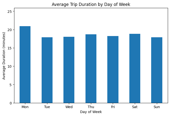
Analysis of average trip durations across the days of the week revealed subtle but consistent patterns in rider behavior. Monday stood out with the longest average trip times, suggesting that the start of the workweek may drive longer commutes or travel needs. In contrast, Tuesday through Friday trips tended to cluster around slightly shorter durations, reflecting more regular weekday travel habits. Weekend trips, while comparable in length to weekdays, showed a small dip on Sunday, which may reflect lighter travel activity as people prepare for the week ahead. These insights highlight the importance of incorporating temporal features such as day of week into predictive models, as they capture recurring behavioral patterns that can influence trip duration.
1.3 Feature Importance from RandomForest
Building on the earlier exploratory analysis, which highlighted temporal patterns in trip durations and revealed that missing drop-off locations were associated with unusual trip lengths, I next turned to a more structured way of quantifying which features mattered most. To do this, I trained a baseline Random Forest model on a sample of the dataset, using both numeric and categorical features such as trip distance, pickup and drop-off community areas, time of day, and company information. The resulting feature importance ranking provided a clear confirmation of the earlier observations: trip distance was by far the dominant predictor of duration, with company identifiers and drop-off location information also playing significant roles. Temporal features like hour of day and day of week, which had shown distinct patterns in the EDA, also emerged as relevant contributors.
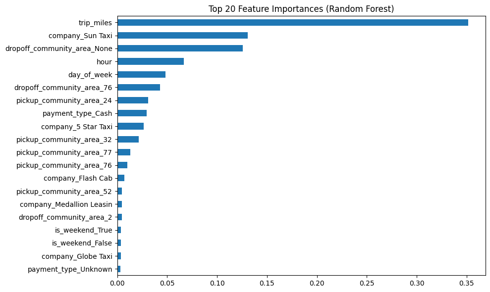
This step created a strong link between the exploratory visual findings and the predictive modeling process, validating that the patterns seen in the data were not just visual curiosities but genuine drivers of trip duration. By grounding feature selection in both intuition and empirical importance scores, I ensured that the pipeline would be built on features that truly carried predictive value. This foundation would later allow for more rigorous experiment tracking and model comparison using MLflow.
2. Experiment Tracking with MLflow
With a solid understanding of the data and a baseline model highlighting key feature importance, the next step in the pipeline was to formalize and track model development using MLflow. Rather than relying on ad-hoc experiments, I built a reproducible framework for training and comparing multiple regression models using a consistent preprocessing pipeline.
To do this, I set up MLflow locally using a lightweight SQLite backend (mlflow.db) and began experimenting with two models: RandomForestRegressor and XGBoostRegressor. For each run, I tracked key performance metrics including MAE along with the model parameters. The MLflow UI made it easy to view these runs side by side and compare their performance in a centralized interface. Among the two, Random Forest clearly outperformed XGBoost across all key metrics, which made it the natural choice for my first candidate model.
To build momentum for the later stages of the pipeline, I went a step further and registered the Random Forest model in the MLflow Model Registry, enabling future access for deployment. While this stage was focused more on experimenting manually, it laid the groundwork for the next part of the project — integrating the training and logging process into a fully automated workflow using Mage.
3. Automated Training with Mage
With my initial MLflow experiments complete and the Random Forest model emerging as the top performer, I moved the workflow into a more automated and production-friendly setup using Mage, an open-source data orchestration tool. This marked the transition from manual experimentation to a modular and maintainable pipeline designed to scale, retrain, and log models dynamically with minimal developer effort.
Mage allowed me to define my ML pipeline as a Directed Acyclic Graph (DAG), where each step — from data preparation to model registration — was broken down into separate, reusable blocks. The pipeline begins with a training_set block that loads and prepares the dataset. From there, a load_models block dynamically defines the models to be tested (e.g., RandomForest, GradientBoosted, LinearRegression), which are then passed into a hyperparameter_tuning block. This block uses MLflow to log all metrics and parameters while tuning each model independently.
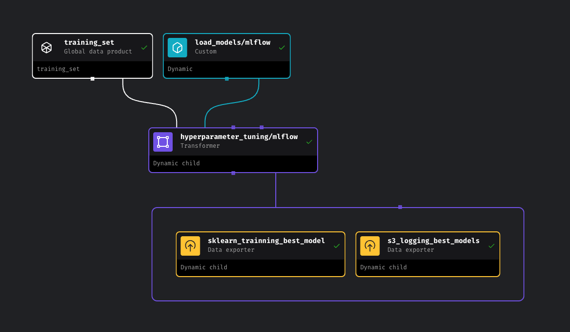
By orchestrating the pipeline this way, I achieved repeatable training runs, automated model selection, and seamless integration with both MLflow’s model registry and S3-based artifact storage. The best model (RandomForest) was automatically registered and promoted to the Production stage in MLflow, while other models were still tracked but not deployed.
This Mage-based approach significantly improves workflow transparency and scalability, especially for future extensions such as retraining on new data or swapping in additional model types. It also decouples logic across different parts of the pipeline, making maintenance and updates much easier.
4. Batch Model Deployment & Real-Time Monitoring
Once the best-performing model (Random Forest) was selected and registered, the final stage of the pipeline focused on batch deployment — simulating realistic taxi ride predictions and monitoring outputs in real time. Unlike real-time APIs, this approach emphasizes scheduled inference, where predictions are made periodically and stored for later analysis.
The system is built using Flask, Prefect, MLflow, PostgreSQL, and Grafana, forming a tightly integrated environment for scheduled batch prediction and dashboard observability. Every few minutes, a Prefect flow generates synthetic yet realistic ride data — based on historical pickup and drop-off patterns — and runs predictions using the production model pulled directly from the MLflow model registry. Each prediction includes metadata such as fare, trip distance, and a UUID-based trip ID. These are logged into a PostgreSQL database and later visualized through a live Grafana dashboard.
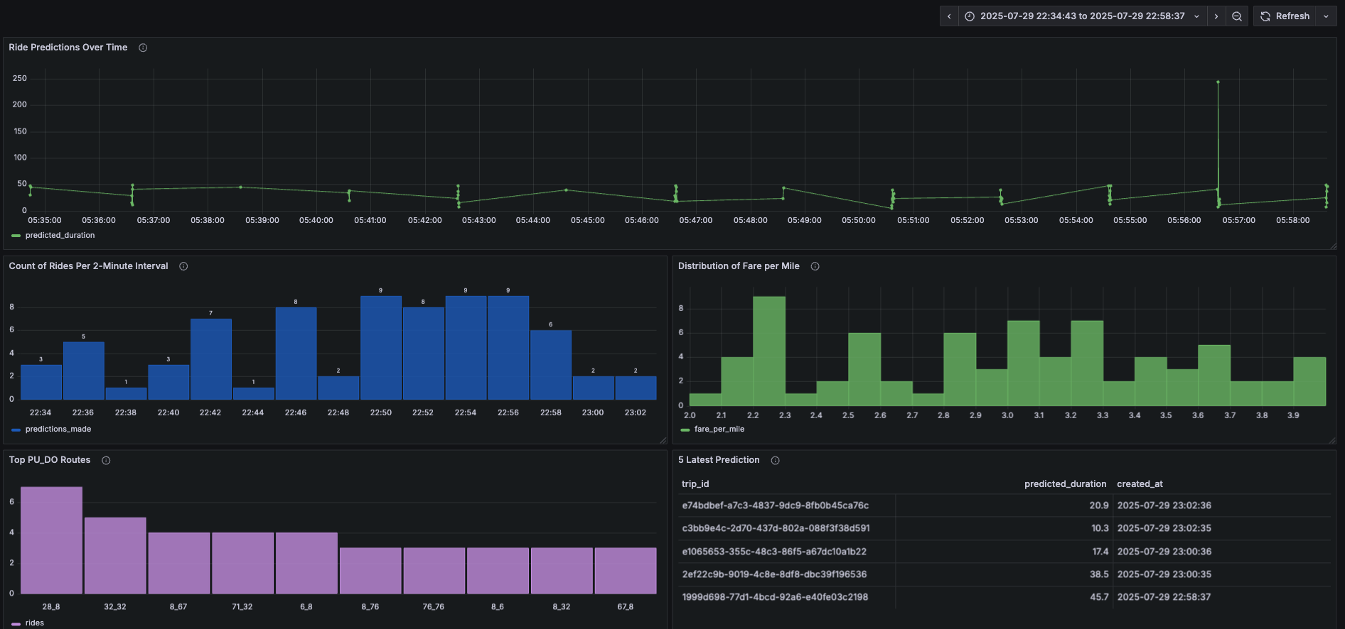
To emulate real-world load and timing, the system was configured to randomly generate between 1 and 10 ride predictions every 2 minutes. This not only tests the system under fluctuating workloads but also provides continuous signals for evaluating model behavior. The dashboard includes key panels such as:
- Ride Predictions Over Time
- Count of Rides per 2-Minute Interval
- Distribution of Fare per Mile
- Top Pickup/Dropoff Routes
- Latest 5 Predictions Table
All infrastructure runs via Docker Compose, which provisions Grafana, PostgreSQL, and Adminer for easy local development and monitoring. This stage brings everything full circle — not just training and deploying a model, but building an ecosystem that can run, log, and monitor machine learning in a production-like setting. It demonstrates how batch inference can be used to simulate real-world scenarios and maintain visibility into model performance through automated pipelines and dashboards.
5. Model Monitoring with Evidently, Grafana, and PostgreSQL
After deployment, maintaining a reliable machine learning system requires more than just accurate predictions — it demands visibility. In the final stage of my Chicago Taxi MLOps pipeline, I set up a robust monitoring system to track data quality, drift, and model behavior in production over time. This part of the project reflects real-world challenges in ML observability, where even the best models can degrade silently if not actively watched.
5.1 Daily Monitoring with Evidently
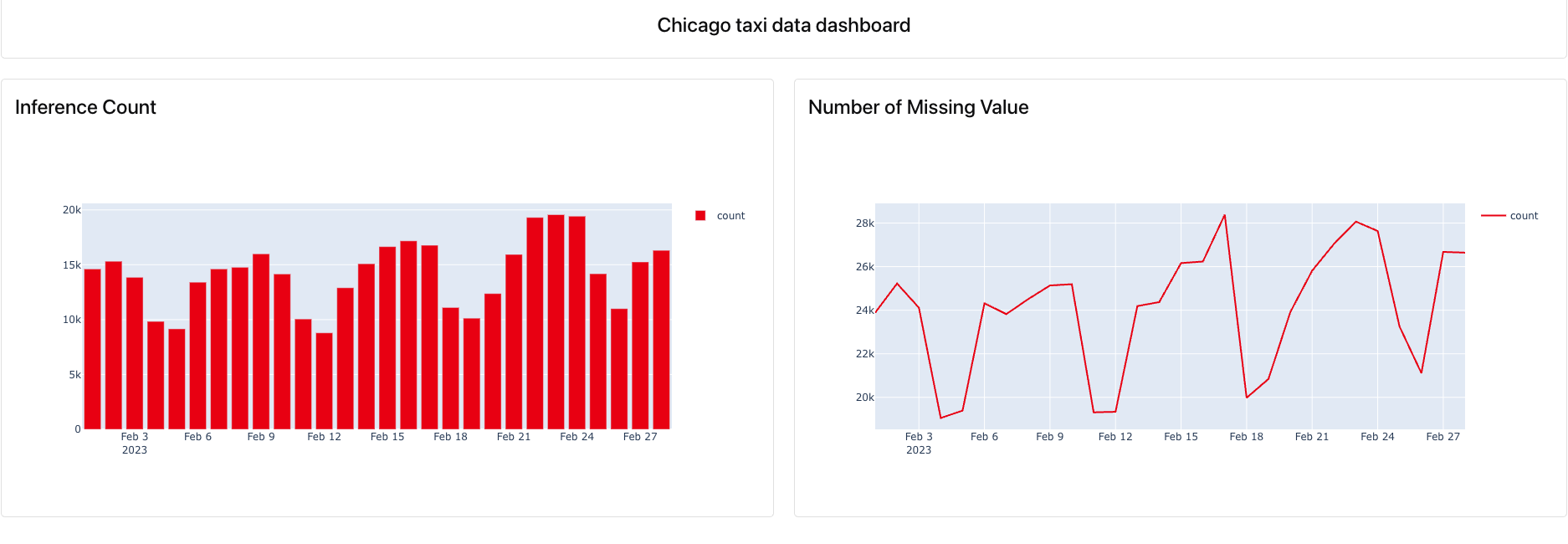
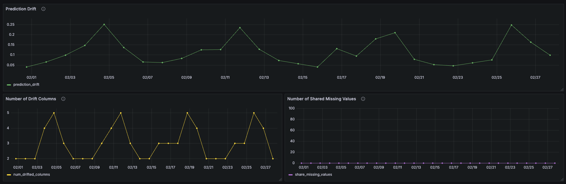
To begin with, I used Evidently to generate automated daily reports comparing the current batch predictions (February) against a historical reference set (January). These reports helped assess:
- Prediction drift, to identify changes in the model’s output distribution.
- Feature drift, to detect changes in input distributions.
- Missing value trends, to catch data pipeline issues early. The reports were created using Python scripts and scheduled to run periodically. For a more interactive experience, the Evidently UI was also launched to explore metrics over time.
- Inference Count per Day
- Prediction Drift Score
- Number of Drifted Features
- Missing Value Distribution
5.2 Real-Time Dashboarding with Grafana + PostgreSQL
To visualize predictions in real time, I logged batch inference outputs to a PostgreSQL database, and connected it to Grafana for dashboarding. The dashboard pulls live metrics such as:
5.3 Why Monitoring Matters
This monitoring infrastructure adds a layer of trust and resilience to the deployed system. Instead of waiting for failures, it allows proactive identification of issues like data anomalies, model degradation, and feature drift — which are common in dynamic environments like urban ride data. By combining Evidently for reporting and Grafana for visualization, the pipeline achieves a high level of observability without complex overhead.
6. Best Practices, Testing, and Development Workflow
To wrap up the project, I ensured the entire pipeline was built with maintainability and reproducibility in mind — key principles in any production-grade machine learning system. This final section focuses on the best practices applied throughout the project to keep the codebase clean, reliable, and easy to extend.
The best-practice part includes unit tests, integration tests, code formatting, and automation scripts to streamline development. Unit tests validate individual components, such as data preprocessing functions, while integration tests ensure the entire pipeline — including the Flask prediction API — behaves as expected. This layered testing approach minimizes regressions and builds confidence when making changes.
To enforce coding standards, I used Black for automatic code formatting and Ruff for linting, helping catch potential issues and maintain code readability. A Makefile ties everything together, allowing developers (or CI pipelines) to execute tasks like testing, linting, cleaning, and running the app with a single command.
Additionally, the system loads model artifacts from AWS S3 via MLflow, ensuring the deployed Flask app always uses the latest version of the production model from the registry.
| Command | Description |
|---|---|
make install |
Install all dependencies via Pipenv |
make format |
Format code using Black |
make lint |
Lint code using Ruff |
make unit-test |
Run unit tests only |
make integration-test |
Run integration tests only |
make test |
Run all tests |
make run |
Start the Flask app locally |
make clean |
Remove temporary files and caches |
6.1 Why this Matter?
Testing and code quality are often overlooked in ML projects, but they’re critical for long-term success. This structure ensures that updates to the model or pipeline don’t break downstream functionality and that future collaborators can easily contribute to the codebase. With clear test coverage, consistent formatting, and automation in place, this MLOps pipeline doesn’t just work — it’s built to last.
7. Conclusion
This project showcases a robust end-to-end MLOps pipeline designed for predictive modeling using the Chicago Taxi dataset. From data ingestion and transformation to model training, evaluation, and deployment, each stage was crafted with scalability, maintainability, and reproducibility in mind.
To ensure transparency and traceability, early experiments with XGBoost and Random Forest were tracked using MLflow, leading to the selection of Random Forest as the most performant model. This model was later incorporated into a workflow orchestrated with Mage, enabling automation and efficient handling of pipeline tasks.
The final component emphasizes development best practices. A dedicated test framework using pytest was implemented for both unit and integration testing, supported by formatting (black), linting (ruff), and automated tasks via Makefile. These tools together promote clean, production-ready code and significantly streamline collaboration and ongoing maintenance.
Overall, this project not only demonstrates technical competency in model development and deployment but also reflects a strong understanding of software engineering principles essential for building reliable and scalable ML systems.
THANK YOU FOR READING!